3C277.1 e-MERLIN: Part 2 Imaging
This is the CASA v5 version of this tutorial! If you don't mean to be here, got back to the Data Reduction workshop page to get the CASA v6 tutorials.
This imaging tutorial follows the calibration tutorial of 3C277.1. IMPORTANT If you have not conducted part 1 (or it went badly!), you will need to download the associated scripts and data from the 3C277.1 workshop homepage.
Either way you should have the following files in your current directory before you start
3C277.1_imaging_outline.py- calibration script equivalent of the guide3C277.1_imaging.py.tar.gz- compressed script for part 2 in case you get stuck1252+5634.ms.tar.gz- measurement set
Table of Contents
- Initial inspection of 1252+5634.ms (step 1)
- First image of 3C277.1 (step 2)
- Inspect to choose interval for initial phase self-calibration (step 3)
- Derive phase self-calibration solutions (step 4)
- Apply first phase solutions and image again (step 5)
- Phase-self-calibrate again (step 6)
- Apply the solutions and re-image (step 7)
- Choose solution interval for amplitude self-calibration (step 8)
- Amplitude self-cal (step 9)
- Apply amplitude and phase solutions and image again (step 10)
- Reweigh the data according to sensitivity (step 11)
- Try multi-scale clean (step 12)
- Taper the visibilities during imaging (step 13)
- Different imaging weights: Briggs robust (step 14)
- Summary and conclusions
The task names are given below. You need to fill in one or more parameters and values where you see ***. Use the help in CASA, e.g. for tclean.
taskhelp                        # list all tasks
inp(tclean)                     # possible inputs to task
help(tclean)                    # help for task
help(par.cell)                  # help for a particular input (only for some parameters)
This tutorial will be done interactively and in script format. You should use the interactive CASA prompt to run the commands. Once you have executed the task correctly, add the correct commands into the 3C277.1_imaging_outline.py script. Alternatively, you can add the correct parameters directly into the script and excute the code step by step (it's up to you!)
1. Initial inspection of 1252+5634.ms (step 1)
Extract 1252+5634.ms using tar -xvzf 1252+5634.ms. If you have already done part 1, you don't need to do this!
Important: If you have already tried this tutorial, but want to start from scratch again, you can either use clearcal(vis=1252+5634.ms), or, if you think you have really messed it up, delete it and re-extract the tar file).
Start CASA, list the contents of the measurement set (writing the output to a list file for future reference).
listobs(vis='**',
		listfile='**')
Make a note of the frequency and the number of channels per spw.
You've done this in part 1, but it's always good to practice! Plot amplitude against uv distance, averaging all channels per spw (just for correlations RR,LL, here and for future plotting).
plotms(vis=target+'.ms',
	   xaxis='**',
	   yaxis='**',
	   correlation='**',
	   avgchannel='**',
	   coloraxis='spw',
	   overwrite=True)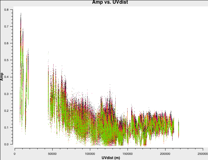
Note the longest baseline $uv$ distance.
Now, in plotms, using the axes tab, select data in the Column drop-down menu and re-plot. The model should be the default flat $1\,\mathrm{Jy}$, if you have not done any imaging yet.
2. First image of 3C277.1 (step 2)
Work out the imaging parameters.
max_B = ***                                # max. baseline from uv plot (in metres)
wavelength = ***                           # approximate observing wavelength (in metres) - listobs gives the frequency.
theta_B= 3600.*degrees(wavelength/max_B)   # convert from radians to degrees and thence to arcsec
To find a good cell size, take theta_B/5 rounded up to the nearest milliarcsecond. To find a good image size, look at Ludke et al. 1998 page 5, 3C277.1 and estimate the size of that image, in pixels. Due to the sparse uv coverage of e-MERLIN and thus extended sidelobes, the ideal image size is at least twice that in order to help deconvolution. As this is quite a small data set, you can pick a power of two which is larger than that.
tclean(vis='1252+5634.ms',
	   imagename='1252+5634_1.clean',
	   cell='**arcsec',
	   niter=700,
	   imsize='***',
	   interactive=True)
Set a mask round the obviously brightest regions and clean interactively, mask new regions or increase the mask size as needed. Stop cleaning when there is no real looking flux left.
Have a look at the image in the viewer (by typing viewer into CASA). If you start the viewer and click on an image to load, the synthesised beam is displayed, and is about $70\times50\,\mathrm{mas}$ for this image.
Measure the noise and peak. This set of boxes are for a 512-pixel image size, change if you used a different size.
rms1=imstat(imagename=target+'_1.clean.image',
			box='10,400,199,499')['rms'][0]
peak1=imstat(imagename=target+'_1.clean.image',
			box='10,10,499,499')['max'][0]

print(target+'_1.clean.image rms %7.3f mJy' % (rms1*1000.))
print(target+'_1.clean.image peak %7.3f mJy/bm' % (peak1*1000.))
I managed to get a peak brightness of $S_p\sim 151.925\,\mathrm{mJy\,beam^{-1}}$ and an r.m.s. of $\sigma \sim 1.896\,\mathrm{mJy\,beam^{-1}}$. This corresponds to a signal-to-noise ratio ($\mathrm{S/N}$) of around 80. You should find that your S/N should be similar and is within the range of 70-120. The r.m.s. is highly dependent on what box you use as the pixel noise distribution is highly non-gaussian (due to residual calibration errors).
The following command illustrates the use of imview to produce reproducible images. This is optional but is shown for reference. You can use the viewer interactively to decide what values to give the parameters. NB If you use the viewer interactively, make sure that the black area is a suitable size to just enclose the image, otherwise imview will produce a strange aspect ratio plot.
imview(raster={'file': '1252+5634_1.clean.image',
       'colormap':'Rainbow 2',
       'scaling': -2,
       'range': [-1.*rms1, 40.*rms1],
       'colorwedge': True},
       zoom=2,
       out='1252+5634_1.clean.png')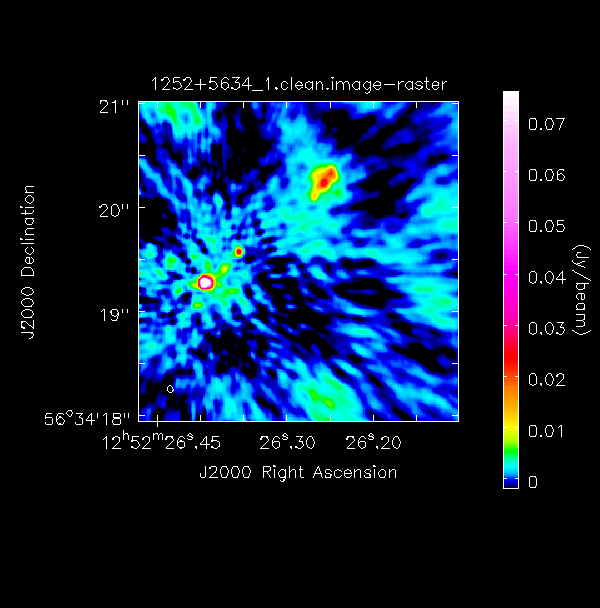
In preparation for self-calibration, we want to inspect our model that we shall use to derive solutions. tclean can do this automatically if you set the savemodel parameter, but sometimes models do not get saved. We shall do this now manually using the ft command.
ft(vis='***',
   model='***',
   usescratch=True)
With the $\texttt{MODEL}$ column now filled, use plotms as in step 1 to plot the model against $uv$ distance.
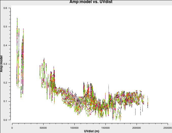
You can also plot data-model which shows that there are still many discrepancies.
3. Inspect to choose interval for initial phase self-calibration (step 3)
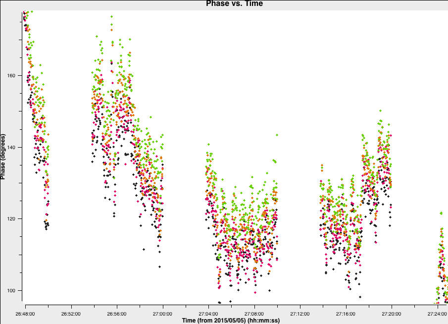
It is hard to tell the difference between phase errors and source structure in the visibilities, but it helps to balance between choosing a longer interval to optimise S/N, and too long an interval (if possible the phase changes by less than a few tens of degrees). The phase will change most slowly due to source structure on the shortest baseline, Mk2&Pi, but you should also check that the longest baselines (to Cm) to ensure that there is enough S/N. Plot phase against time, averaging all channels per spw (see listobs for the number of channels).
plotms(vis='***'',
	   xaxis='***',
	   yaxis='***',
	   antenna='***',
	   correlation='***',
	   avgchannel='**',
	   coloraxis='spw',
	   plotfile='',
	   overwrite=True)
The plot below shows a zoom on a few scans. The chosen solution interval should also ideally fit an integral number of times into each scan. It is also a good idea not to use too short a solution interval for the first model. This is because the model may not be very accurate, so you don't want to constrain the solutions too tightly.
4. Derive phase self-calibration solutions (step 4)
Let's use gaincal to derive solutions
gaincal(vis=target+'.ms',
		calmode='***',          # phase only
		caltable='target.p1',
		field=target,
		solint='***',           # about half a scan duration
		refant=antref,
		minblperant=2,minsnr=2) # These are set to lower values than the defaults which are for arrays with many antennas
Check the terminal and logger; there should be no (or almost no) failed solutions.
Plot solutions
plotcal(caltable='target.p1',xaxis='time',
		plotrange=[-1,-1,-180,180],
		iteration='antenna',yaxis='phase',subplot=321,
		poln='L')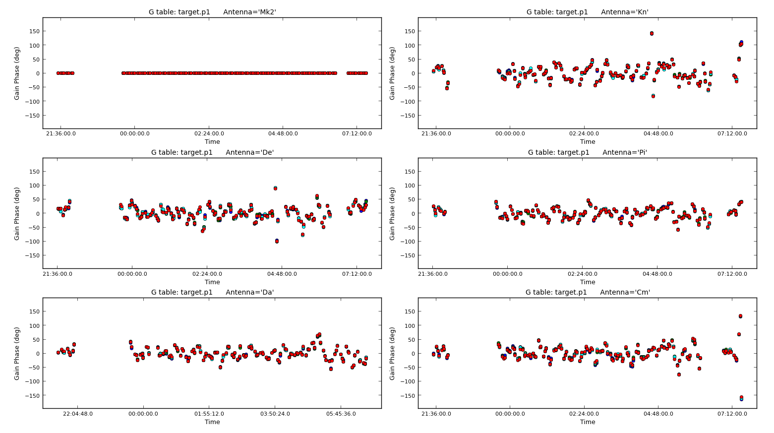
Repeat for the other polarisation. The corrections should be coherent, as they are, and represent the difference caused by the different atmospheric paths between the target and phase-ref, but they may also have a spurious component if the model was imperfect. The target is bright enough that a shorter solution interval could be used. So, these solutions are applied, the data re-imaged and the corrections refined iteratively.
5. Apply first phase solutions and image again (step 5)
Let's continue by applying these solutions to the measurement set. This may take a minute as the $\texttt{CORRECTED}$ data column needs to be generated.
applycal(vis='***',
		 gaintable='***') # enter the name of the MS and the gaintable
With these corrections applied let's use tclean, as before, but you might be able to do more iterations as the noise should be lower.
os.system('rm -rf 1252+5634_p1.clean*')
tclean(vis='1252+5634.ms',
	   imagename='1252+5634_p1.clean',
	   cell='**arcsec',
	   niter=1000,  # stop before this if residuals reach noise
	   deconvolver='clark',
	   imsize='***',
	   interactive=True)
Use imstat to find the rms again and viewer to inspect the image, and plot it if you want. Using the same boxes as before, I managed to get $S_p \sim 169.130 \,\mathrm{mJy\,beam^{-1}}$ and $\sigma \sim 0.807\,\mathrm{mJy\,beam^{-1}}$. This is a massive $\mathrm{S/N}$ increase to $\sim210$.
Important: A key indicator if self-calibration that self-calibration is going correctly is to observe the increase in $\mathrm{S/N}$ per iteration. DO NOT rely on just measuring the rms as the self-calibration model could be bad and is artificially reducing all amplitudes!
Again, let's Fourier Transform this improved model back into the measurement set.
ft(vis='***',
   model='***', # remember to use the new model!
   usescratch=True)
6. Phase-self-calibrate again (step 6)
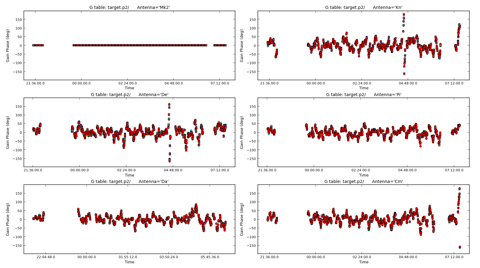
Now that the model is better, use a shorter solution interval. Heuristics suggest that 30s is usually about the shortest worth using, because the atmosphere is reasonably stable on these baseline lengths at this frequency.
Run gaincal as before, but reduce the solint to 30s and write a new solution table (the new model will be used).
os.system('rm -rf target.p2')
gaincal(vis='1252+5634.ms',
		calmode='***',
		caltable='target.p2',
		field=target,
		solint='***',
		refant=antref,
		minblperant=2,minsnr=2)
Plot the solutions
7. Apply the solutions and re-image (step 7)
Use applycal as before, just changing the name of the gaintable to the new one.
applycal(vis='1252+5634.ms',
		 gaintable='***')
From listobs, the total bandwidth is almost 10% of the frequency, which is enough to take the spectral index into account. Cotton et al. (2006) finds a spectral index varies from -0.1 in the core to as steep as -1.
listobs showed the total bandwidth is 4817 to 5329 MHz, i.e. for flux density $S$, $S_{4817}/S_{5329} = (4817/5329)^{-1}$ or about 10%. The improved S/N gives much greater accuracy. Thus, in order to image properly and produce an accurate image to amplitude self-calibrate all spectral windows, multi-term multi-frequency synthesis (MT-MFS) imaging is used. This solves for the sky model changing across frequency.
Make sure you clean till as much target flux as possible has been removed into the model - you can increase the number of iterations interactively if you want.
tclean(vis='1252+5634.ms',
	   imagename='1252+5634_p2.clean',
	   cell='***arcsec',
	   niter=1000, # stop before this if residuals reach noise
	   imsize=***,
	   deconvolver='mtmfs',
	   nterms=2, # Make spectral index image w/ linear fit
	   interactive=True)
Use ls to see the names of the image files created. The image name is 1252+5634_p2.clean.image.tt0.
If we check the image using the same boxes as before, I get $S_p \sim 171.360 \,\mathrm{mJy\,beam^{-1}}$ and $\sigma \sim 0.443\,\mathrm{mJy\,beam^{-1}}$. This is another large $\mathrm{S/N}$ increase to $\sim 387$.
Let's put the model we derived into the visibilities. To encode the frequency dependence of the source we need to include both terms of the model (i.e. the tt0 and tt1 models).
ft(vis='1252+5634.ms',
   model=['***.model.tt0','***.model.tt1'], # model images from the MTMFS images,
   nterms=**, # same as tclean!
   usescratch=True)
8. Choose solution interval for amplitude self-calibration (step 8)
Plot amplitude against time in order to choose a suitable solution interval.
plotms(vis='1252+5634.ms',
	   xaxis='***',
	   yaxis='***',
	   ydatacolumn='***',
	   antenna='Mk2&**',
	   correlation='**,**',
	   avgchannel='**',
	   coloraxis='spw')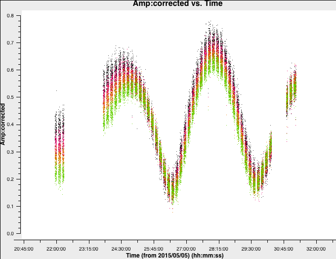
The amplitudes change more slowly than phase errors and a suitable solint is a few times longer than for phase.
9. Amplitude self-cal (step 9)
In gaincal, the previous gaintable with short-interval phase solutions will be applied, to allow a longer solution (averaging) interval foramplitudee self-calibration. Set up gaincal to calibrate amplitude and phase, with a longer solution interval, and the same refant etc. as before.
os.system('rm -rf target.ap1')
gaincal(vis='1252+5634.ms',
calmode='***', # amp and phase
caltable='target.ap1',
field='1252+5634',
solint='***',
refant='Mk2',
gaintable='***', # the phase table should be applied
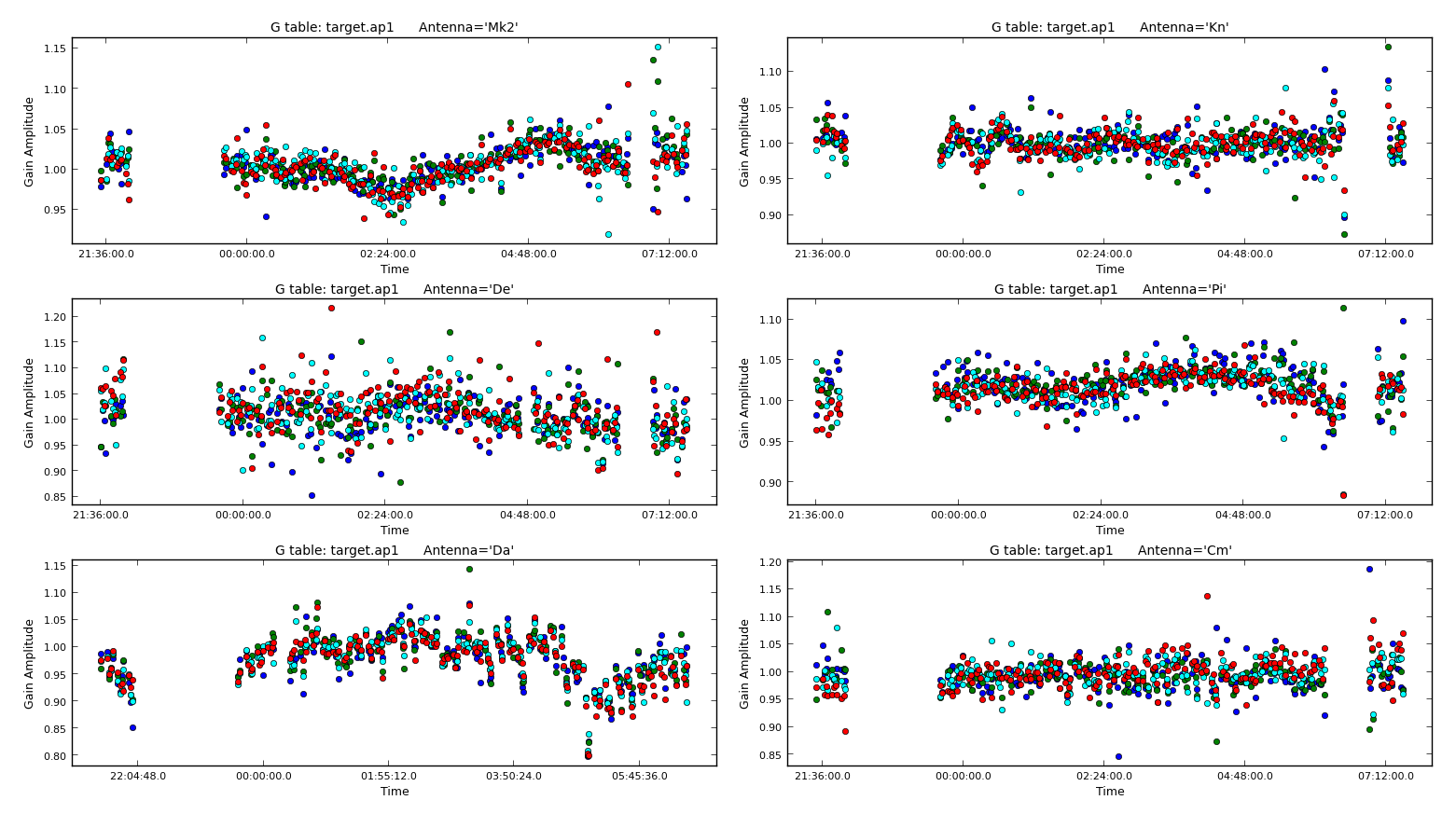
minblperant=2,minsnr=2)Plot the solutions. They should mostly be within about 20% of unity. A few very low points implies some bad data (high points). If the solutions are consistently much greater than unity then the model is missing flux.
10. Apply amplitude and phase solutions and image again (step 10)
Use applycal to apply the short-interval phase solution table and the amplitude and phase table you have just created.
applycal(vis=target+'.ms',
		 gaintable=['**','**'])
Clean the image again, as before and inspect.
tclean(vis='1252+5634.ms',
	   imagename='1252+5634_ap1.clean',
	   cell='***arcsec',
	   niter=1500, # stop before this if residuals reach noise
	   imsize=***,
	   deconvolver='mtmfs',
	   nterms=**, # Make spectral index image
	   interactive=True)
Again, with the same boxes, I get $S_p \sim 171.717 \,\mathrm{mJy\,beam^{-1}}$ and $\sigma \sim 0.174\,\mathrm{mJy\,beam^{-1}}$. This now corresponds a huge $\mathrm{S/N}\sim 987$. The key message with self-calibration is to increase the S/N of your observations by removing calibration errors whilst not constraining your visibilities to the model. Due to the number of free parameters, you need to use an iterative approach to obtain the true source structure! It takes practice to know what's right and wrong.
11. Reweigh the data according to sensitivity (step 11)
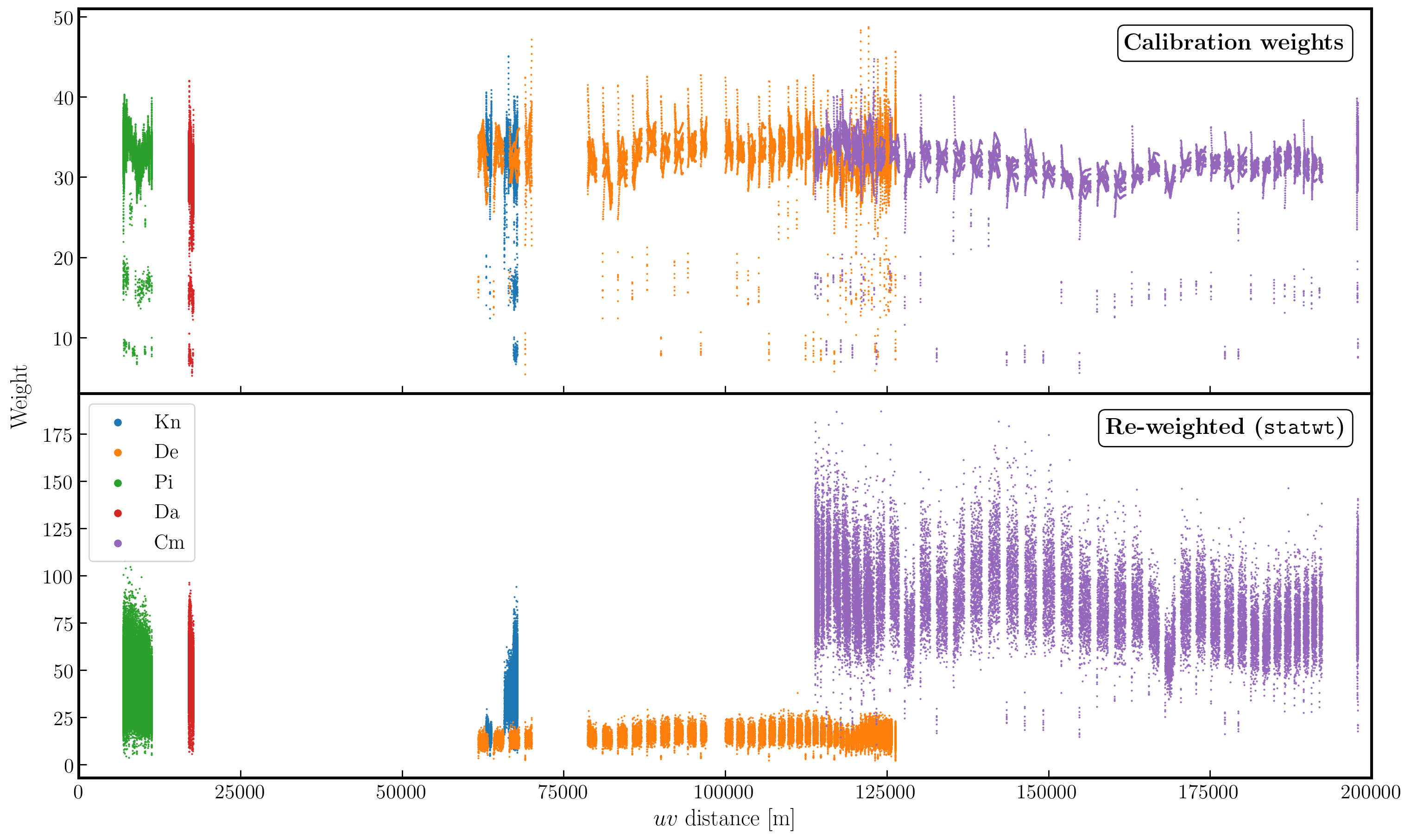
Often, especially for heterogeneous arrays, the assigned weighting is not optimal for sensitivity. For example, the Cambridge (Cm) telescope is more sensitive, therefore, to get the optimal image must be given a larger weight than the other arrays.
To recalculate the optimal weights we use the task statwt calculates the weights based on the scatter in small samples of data. Note that the original data are overwritten, so you might want to copy the MS to a different name or directory first.
There are alot of options here, but we are just going to use the default options. You can try with different weightings if you'd like.
statwt(vis='***')
In the plot below, we show the weights before (top panel) and after re-weighting (bottom panel) on the baselines to our refant (Mk2). As you can see, the telescopes have similar weights despite Cm being more sensitive. With the use of statwt, the weights now reflect the sensitivities, and have also adjusted some errant weights which were low before.
12. Try multi-scale clean (step 12)
Let's image the re-weighted data using multiscale clean, which instead assumes that the sky can be represented by a bunch of Gaussians rather than delta functions. Have a look at the help for tclean, which suggests suitable values of the multiscale parameter.
tclean(vis='1252+5634.ms',
	   imagename='1252+5634_ap1_multi.clean',
	   cell='***arcsec',
	   niter=***, # stop before this if residuals reach noise
	   imsize=***,
	   deconvolver='***', # find the multiscale option (mtmfs does it!)
	   scales=[**,**,**], # add scales to use (in pixels)
	   nterms=*, # also want mtmfs!
	   interactive=True)
You will find that the beam is now slightly smaller (I got $60\times44\,\mathrm{mas}$) as the longer baselines have more weight, so the peak is lower. I got $S_p \sim 151.086 \,\mathrm{mJy\,beam^{-1}}$ and $\sigma \sim 0.076\,\mathrm{mJy\,beam^{-1}}$.
13. Taper the visibilities during imaging (step 13)
Experiment with changing the relative weights given to longer baselines. Applying a taper reduces this, giving a larger synthesised beam more sensitive to extended emission. This just changes the weights during gridding for imaging, no permanent change to the uv data. However, strong tapering increases the noise.
Look at the uv distance plot and choose an outertaper (half-power of Gaussian taper applied to data) which is about 2/3 of the longest baseline. Units are wavelengths, so calculate that or plot amp vs. uvwave.
tclean(vis='1252+5634.ms',
	   imagename='1252+5634_ap1_taper.clean',
	   cell='***arcsec',
	   niter=1500, # stop before this if residuals reach noise
	   imsize=***,
	   deconvolver='***', ## same as for multiscale
	   uvtaper=['***Mlambda'],  ## ~2/3 of the longest baseline
	   scales=[**,**,**], ## same as for multiscale
	   nterms=*,
	   interactive=True)
Inspect the image and check the beam size. I got a restoring beam of $74\times61\,\mathrm{mas}$, $S_p \sim 188.140\,\mathrm{mJy\,beam^{-1}}$ and $\sigma \sim 0.105\,\mathrm{mJy\,beam^{-1}}$.
14. Different imaging weights: Briggs robust (step 14)
Experiment with changing the relative weights given to longer baselines. Default natural weighting gives zero weight to parts of the uv plane with no samples. Briggs weighting interpolates between samples, giving more weight to the interpolated areas for lower values of robust. For an array like e-MERLIN with sparser sampling on long baselines, this has the effect of increasing their contribution, i.e. making the synthesised beam smaller. This may bring up the jet/core, at the expense of the extended lobes. Low values of robust increase the noise. You can combine with tapering or multiscale, but initially remove these parameters.
tclean(vis='1252+5634.ms',
	   imagename='1252+5634_ap1_robust.clean',
	   cell='***arcsec',
	   niter=1500, # stop before this if residuals reach noise
	   imsize=***,
	   deconvolver='***',
	   nterms=*,
	   weighting='***',
	   robust=**,
	   interactive=True)
I got a beam of $56\times40\,\mathrm{mas}$, $S_p \sim 147.872\,\mathrm{mJy\,beam^{-1}}$ and $\sigma \sim 0.191\,\mathrm{mJy\,beam^{-1}}$
15. Summary and conclusions
To summarise, this workshop can be broadly grouped into two main parts: i) self-calibration and ii) imaging.
We began with a simple phase-reference calibrated data set of our target. Here, the phase and amplitude corrections are valid for our nearby phase calibrator, but crucially only approximately valid for our target. This is because the patch of sky the telescopes are looking through for the target, is not the same as the phase calibrator.
For our target source, the assumption that our source is a simple point source in invalid (as proven by the uv distance plots). This means that, in order to calibrate for the gain differences between the phase cal and target fields, we need to produce a model to calibrate against. The approximate phase and amplitude solutions are just valid enough for us to derive a first order model.
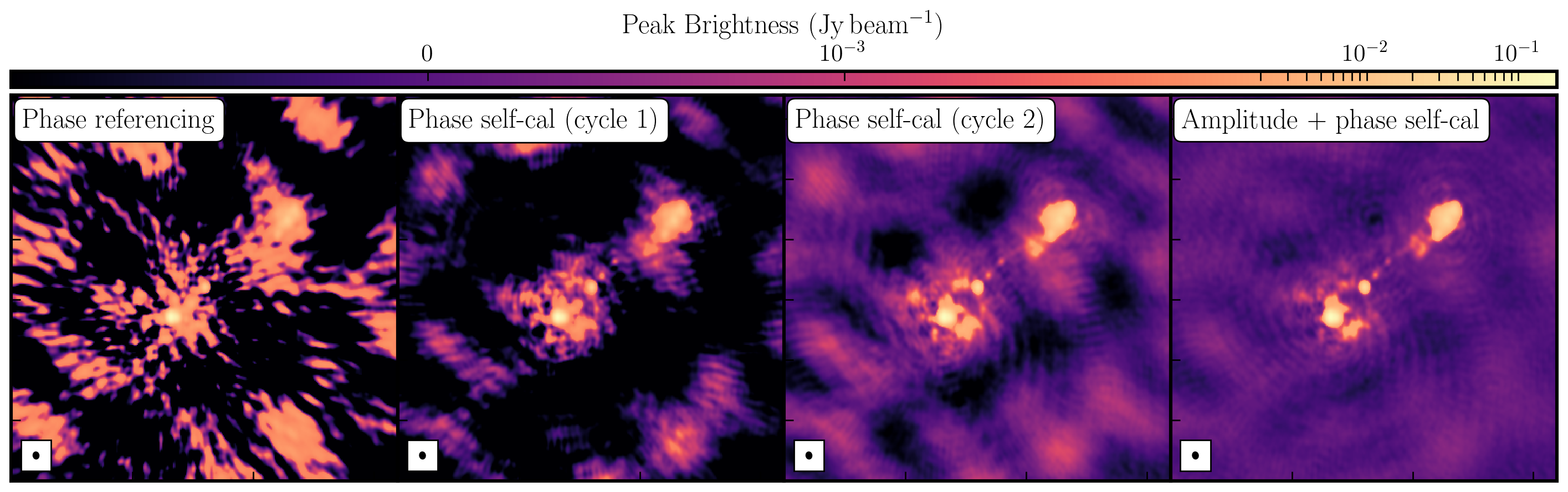
Once we generated a model using deconvolution, the Fourier Transform of these are used to calibrate against. We begin with phase only calibration as this needs less S/N for good solutions. With these corrections applied, we can generate a much better model whose S/N has increased dramatically. This S/N boost can then be used to then calibrate for amplitudes and phases. As a result, we end up with a high dynamic range data set (with a high S/N), where lots of low level source structure has appeared. The following table and plot illustrates this vast improvement.
| Peak Brightness | Noise (r.m.s.) | S/N | |
|---|---|---|---|
| [$\mathrm{mJy\,beam^{-1}}$] | [$\mathrm{mJy\,beam^{-1}}$] | ||
| Phase referencing | 151.925 | 1.896 | 80.129 |
| Phase self-calibration (cycle 1) | 169.130 | 0.807 | 209.579 |
| Phase self-calibration (cycle 2) | 171.360 | 0.443 | 386.817 |
| Amp+phase self-calibration | 171.717 | 0.174 | 986.879 |
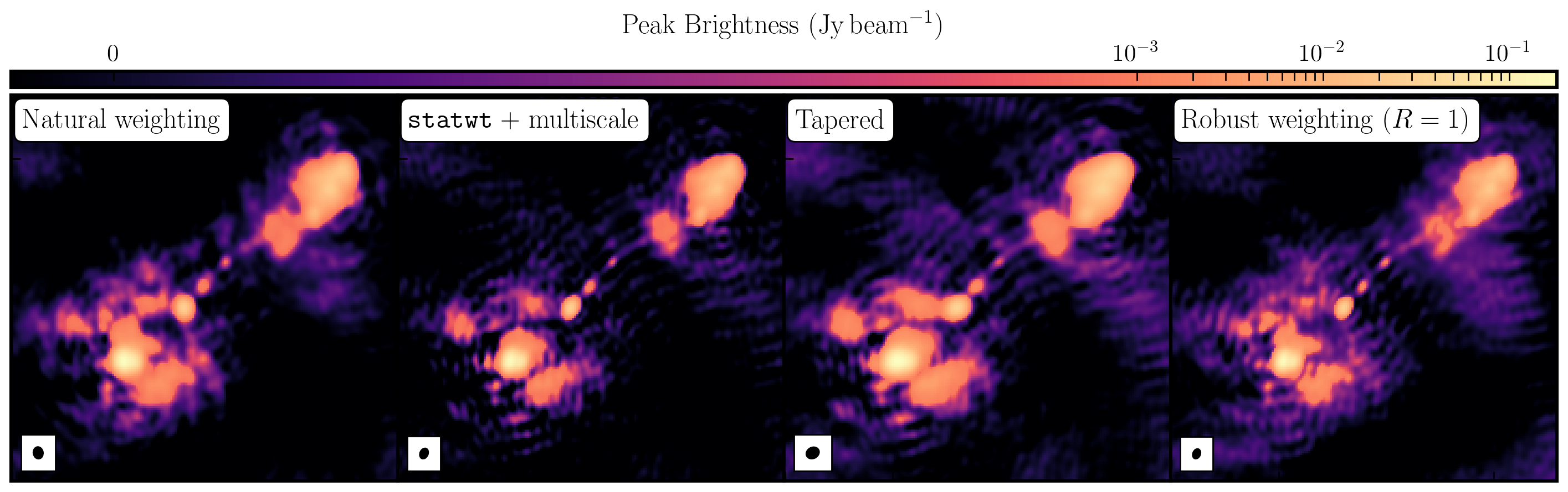
While the first part of this tutorial fixed residual calibration errors associated with approximate gain and phase solutions derived from the phase calibrator, the second part investigated the various imaging techniques which can be used to extenuate features. In the first instance we used statwt to optimally reweigh the data to have maximum sensitivity. We find that the Cm telescope is the most sensitive (as it is 32m wide), but also contains all the long baselines. As a result these long baselines are expressed more when imaging resulting in a higher resolution image than what we've seen before. As a result the peak flux reduces but so did the sensitivity! IN addition, we used multiscale clean to better deconvolve the large fluffy structures which standard clean can struggle with.
The next step that we did was to taper the weights with respect to uv distance. The downweighting of the long baselines means that we are more sensitive to larger structures hence our resolution is lower. However, because of the sensitivity contained in these long baselines, we have a much larger rms.
And finally, we introduced robust weighting schemes. These schemes provide a clear way to achieve intermediate resolutions between naturally weighted and uniformly weighted data.
| Peak Brightness | Noise (r.m.s.) | S/N | Beam size | |
|---|---|---|---|---|
| [$\mathrm{mJy\,beam^{-1}}$] | [$\mathrm{mJy\,beam^{-1}}$] | [$\mathrm{mas\times mas}$] | ||
| Amp+phase self-calibration | 171.717 | 0.174 | 986.879 | 65 $\times$ 53 |
statwt+multiscale |
151.086 | 0.0760 | 1987.974 | 60 $\times$ 44 |
| Tapering | 188.140 | 0.105 | 1791.810 | 74 $\times$ 61 |
| Robust weighting ($R=1$) | 147.872 | 0.191 | 774.199 | 56 $\times$ 40 |