
3C277.1 e-MERLIN: Part 1 Calibration
This is the CASA v6.3 version of this tutorial! If you don't mean to be here, got back to the Data Reduction workshop page to get the CASA v6.5 tutorials.
This guide provides a basic example for calibrating e-MERLIN C-Band (5 GHz) continuum data in CASA. It has been tested in CASA 6.4. It is designed to run using an averaged data set all_avg.ms (1.7 G), in which case you will need at least 5.5 G disk space to complete this tutorial.
If you have a very slow laptop, you are advised to skip some of the plotms steps (see the plots linked to this page instead) and especially, do not use the plotms options to write out a png. This is not used in this web page, but if you run the script as provided, you are advised to comment out the calls to plotms or at least the part which writes a png, see tutors for guidance.
Table of Contents
- Guidance for calibrating 3C277.1 in CASA
- Data inspection and flagging
- Check data: listobs and plotants (step 1)
- Identify 'late on source' bad data (step 2)
- Flag the bad data at the start of each scan (step 3)
- Flag the bad end channels (step 4)
- Identify and flag remaining bad data (step 5)
- Calibration
- Delay calibration (script step 6)
- Derive delay corrections.
- Setting the flux of the primary flux scale calibrator (script step 7)
- Derive the initial bandpass calibration and inspect effects (script step 8)
- Gain calibration (script step 9)
- Time-dependent phase calibration of all calibration sources
- Time-dependent amplitude calibration of all calibration sources
- Determining flux densities of calibration sources (script step 10)
- Improved bandpass calibration (script step 11)
- Derive solutions for all cal sources with improved bandpass table (script step 12)
- Apply final calibrator source solutions and plot phase-ref and target (script step 13)
- Split out target (script step 14)
1. Guidance for calibrating 3C277.1 in CASA
1A. The data and supporting material
For this part of the workshop, we only need four files in total. Please double check that you have the following in your current directory:
all_avg.ms- the data (after conversion to a measurement set).3C286_C.clean.model.tt0- used for fluxscaling of the data set.all_avg.flags.txt- pre-made flagging file to save time3C277.1_cal_outline.py- the script that we shall input values into to calibrate these data.
.tar.gz or .tar) so you need to use tar -xzvf <filename> to untar these.
1B. How to use this guide
This User Guide presents inputs for CASA tasks e.g. gaincal to be entered interactively at a terminal prompt for the calibration of the averaged data and initial target imaging. This is useful to examine your options and see how to check for syntax errors. You can run the task directly by typing gaincal at the prompt; if you want to change parameters and run again, if the task has written a calibration table, delete it (make sure you get the right one) before re-running. You can review these by typing:
# In CASA
!more gaincal.last
This will output something like:
taskname           = "gaincal"
vis                =  "all_avg.ms"
caltable           =  "bpcals_precal.ap1"
...
...

#gaincal(vis="all_avg.ms",caltable="bpcals_precal.ap1",field="1407+284",spw="",intent="",
selectdata=True,timerange="",uvrange="",antenna="",scan="",observation="",msselect="",solint="120s",
combine="",preavg=-1.0,refant="Mk2",minblperant=2,minsnr=2,solnorm=True,gaintype="G",smodel=[],
calmode="ap",append=True,splinetime=3600.0,npointaver=3,phasewrap=180.0,docallib=False,callib="",
gaintable=['all_avg.K', 'bpcals_precal.p1'],gainfield=[''],interp=[],spwmap=[],parang=False)
As you can see in the script, the second format (without '#') is the form to use in the script, with a comma after every parameter value. When you are happy with the values which you have set for each parameter, enter them in the script 3C277.1_cal_outline.py (or whatever you have called it). You can leave out parameters for which you have not set values; the defaults will work for these (see e.g. help(gaincal) for what these are), but feel free to experiment if time allows.
The script already contains most plotting inputs in order to save time. Make and inspect the plots; change the inputs if you want, zoom in etc. There are links to copies of the plots (or parts of plots) but only click on them once you have tried yourself or if you are stuck.
The parameters which should be set explicitly or which need explanation are given below, with ** if they need values.
If you have already plotted the antenna positions with plotants you will have seen that Mk2 has many short baselines which makes it more likely to give good calibration solutions and it makes a good reference antenna (refant).
The input data set all_avg.ms contains five fields:
| eMERLIN name | Common name | Role |
|---|---|---|
| 1252+5634 | 3C277.1 | target |
| 1302+5748 | J1302+5748 | phase reference source |
| 1407+284 | OQ208 | bandpass cal. (usually about 2 Jy at 5-6 GHz) |
| 0319+415 | 3C84 | bandpass, polarisation leakage cal. (usually 10-20 Jy at 5-6 GHz) |
| 1331+305 | 3C286 | flux, polarisation angle cal. (flux density known accurately, see Step 7) |
These data have already been preprocessing from the original raw fits idi files which included the following:
- Conversion from fitsidi to a CASA compatible measurement set.
- Sorted and recalculated the $uvw$ (visibility coordinates), concatenate all data and adjust scan numbers to increment with each source change.
- Averaged every 8 channels and 4s.
2. Data Inspection and Flagging
2A. Check data: listobs and plotants (script step 1)
Check that you have all_avg.ms in a directory with enough space and start CASA.
Enter the parameter in step 1 of the script to specify the measurement set and, optionally, the parameter to write the listing to a text file. Important: To make it easier, the line numbers corresponding to the script 3C277.1_cal_outline.py are included in the excerpts from the script shown in this tutorial.
	listobs(vis=**,
			overwrite=True,
			listfile=**)
Because e-MERLIN stores data for each source in a separate fitsidi file, the sources are listed one by one even though the phase-ref and target scans interleave. So selected entries from listobs, re-ordered by time, show:
Timerange (UTC)          Scan  FldId FieldName             nRows
  SpwIds   Average Interval(s)  #(i.e. RR RL LR LL integration time) 05-May-2015
...
20:02:08.0 - 20:05:08.5     7      0 1302+5748                 2760  [0,1,2,3]  [3.91, 3.91, 3.91, 3.91]    # phase-ref
20:05:11.0 - 20:12:33.5    72      1 1252+5634                 6660  [0,1,2,3]  [3.98, 3.98, 3.98, 3.98]    # target
20:12:36.0 - 20:15:34.5     8      0 1302+5748                 2700  [0,1,2,3]  [3.96, 3.96, 3.96, 3.96]    # phase-ref
...
22:02:04.0 - 22:47:00.5   132      2 1331+305                 40500  [0, 1, 2, 3]  [3.99, 3.99, 3.99, 3.99] # flux scale/pol angle calibrator
22:47:03.0 - 23:29:59.5   133      3 1407+284                 38700  [0, 1, 2, 3]  [3.99, 3.99, 3.99, 3.99] # bandpass calibrator
06-May-2015
07:30:03.0 - 08:29:59.5   134      4 0319+415                 54000  [0, 1, 2, 3]  [4, 4, 4, 4]             # bandpass/leakage calibrator
There are 4 spw:
 SpwID  Name   #Chans   Frame   Ch0(MHz)  ChanWid(kHz)  TotBW(kHz) CtrFreq(MHz)  Corrs
  0      none      64   TOPO    4817.000      2000.000    128000.0   4880.0000   RR  RL  LR  LL
  1      none      64   TOPO    4945.000      2000.000    128000.0   5008.0000   RR  RL  LR  LL
  2      none      64   TOPO    5073.000      2000.000    128000.0   5136.0000   RR  RL  LR  LL
  3      none      64   TOPO    5201.000      2000.000    128000.0   5264.0000   RR  RL  LR  LL
And 6 antennas:
ID   Name  Station       Diam.    Long.         Lat.                 ITRF Geocentric coordinates (m)
  0    Mk2   e-MERLIN:02 24.0 m   -002.18.08.9  +53.02.58.7     3822473.365000  -153692.318000  5085851.303000
  1    Kn    e-MERLIN:05 25.0 m   -002.59.44.9  +52.36.18.4     3859711.503000  -201995.077000  5056134.251000
  2    De    e-MERLIN:06 25.0 m   -002.08.35.0  +51.54.50.9     3923069.171000  -146804.368000  5009320.528000
  3    Pi    e-MERLIN:07 25.0 m   -002.26.38.3  +53.06.16.2     3817176.561000  -162921.179000  5089462.057000
  4    Da    e-MERLIN:08 25.0 m   -002.32.03.3  +52.58.18.5     3828714.513000  -169458.995000  5080647.749000
  5    Cm    e-MERLIN:09 32.0 m   +000.02.19.5  +51.58.50.2     3919982.752000     2651.982000  5013849.826000
Enter one parameter to plot the antenna positions (optionally, a second to write this to a png).
plotants(vis=**, figfile=**)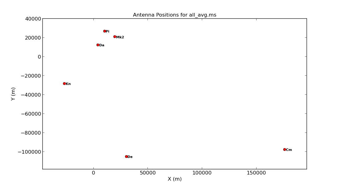
Consider what would make a good reference antenna. Although Cambridge has the largest diameter, it has no short baselines.
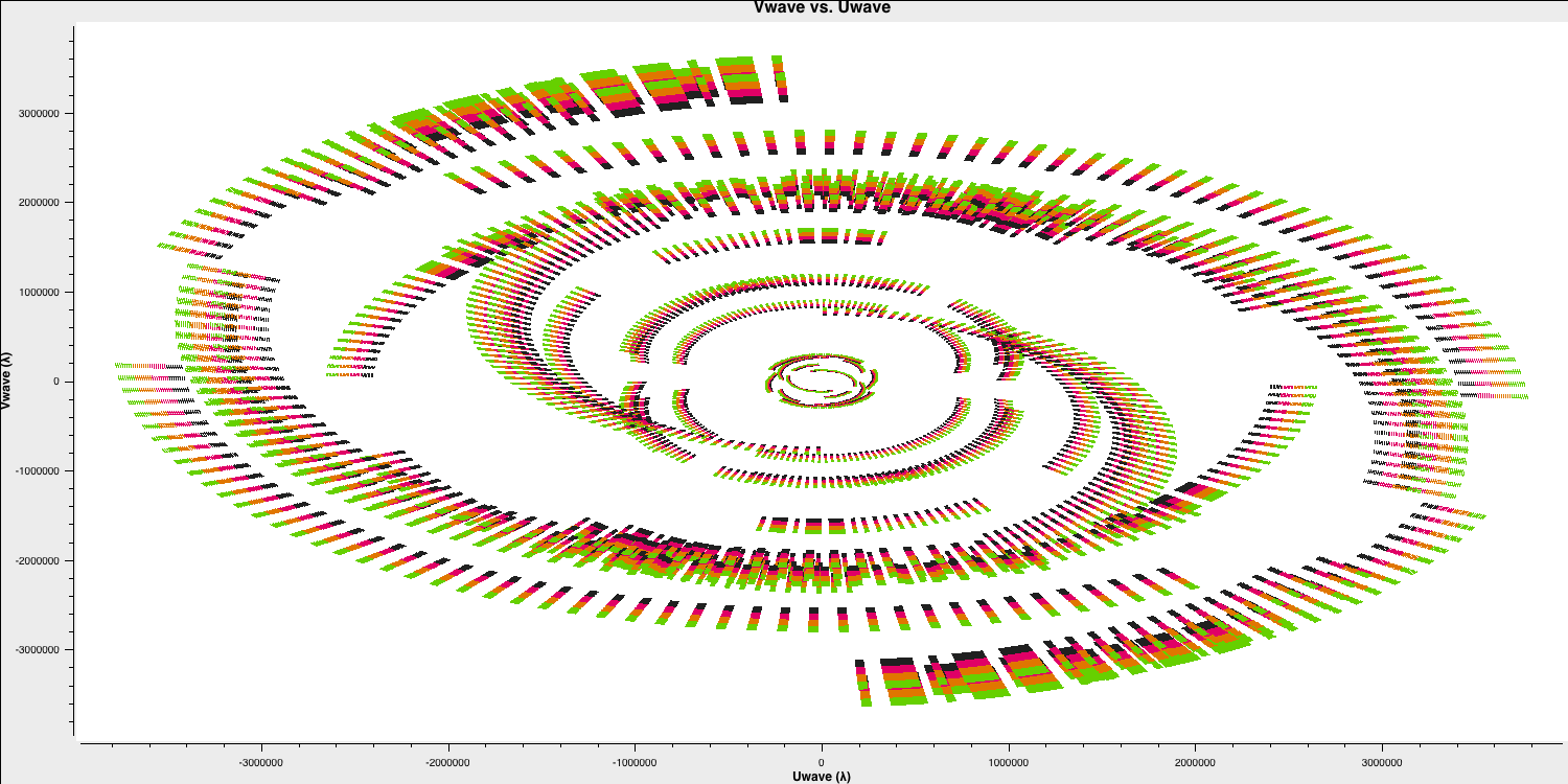
Plot the uv coverage of the data for the phase-reference source. See annotated listobs output above to identify this. You need to enter several parameters but some have been done for you:
	plotms(vis='**',
		   xaxis='**',
		   yaxis='**',
		   coloraxis='spw',
		   avgchannel='8',
		   field='1302+5748',
		   showgui=gui)
Note that we averaged in channels a bit so that this doesn't destroy your computer. If this takes a long time, move on and look at the plot below. The $u$ and $v$ coordinates represent (wavelength/projected baseline) as the Earth rotates whilst the source is observed. Thus, as each spw is at a different wavelength, it samples a different part of the uv plane, improving the aperture coverage of the source, allowing Multi-Frequency Synthesis (MFS) of continuum sources.
If you are happy with your entries, execute step 1 and you should see these two plots in your current directory. Remember we execute a step using the following syntax in the CASA prompt:
runsteps=[1]
execfile('3C277.1_cal_outline.py')
2B. Identify 'late on source' bad data (step 2)
Use plotms to plot the phase-reference source amplitudes as a function of time. Just a few central channels are selected and averaged; enough to give good S/N but not so many that phase errors across the band cause decorrelation (in real life, you might have to experiment with different selections or plot phase vs. channel to make the selection). Some hints on the proper parameter selection are given in the code blocks below.
	plotms(vis='***',
		   field='***',  # phase ref
		   spw='***',    # plot just the inner 3/8 of the channels for each spw (see listobs output)
		   avgchannel=***, # average these channels
		   xaxis='***', yaxis='***',
		   antenna=antref+'&**', # This uses Mk2 as refant for ease of comparison but another with many short baselines could be used.
		   correlation='**,**',  # Just select the parallel hands, since the cross hands (polarised intensity) are much fainter.
		   coloraxis='corr', # Color by baseline or correlation as you prefer
		   showgui=True,
		   overwrite=True, plotfile='')
Once you have inputted the parameters, execute step 2. Note that you can change the parameters interactively once plotms has started.
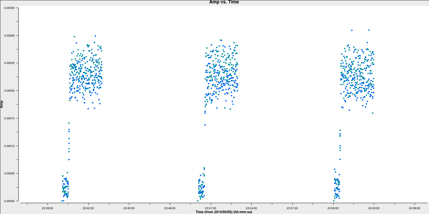
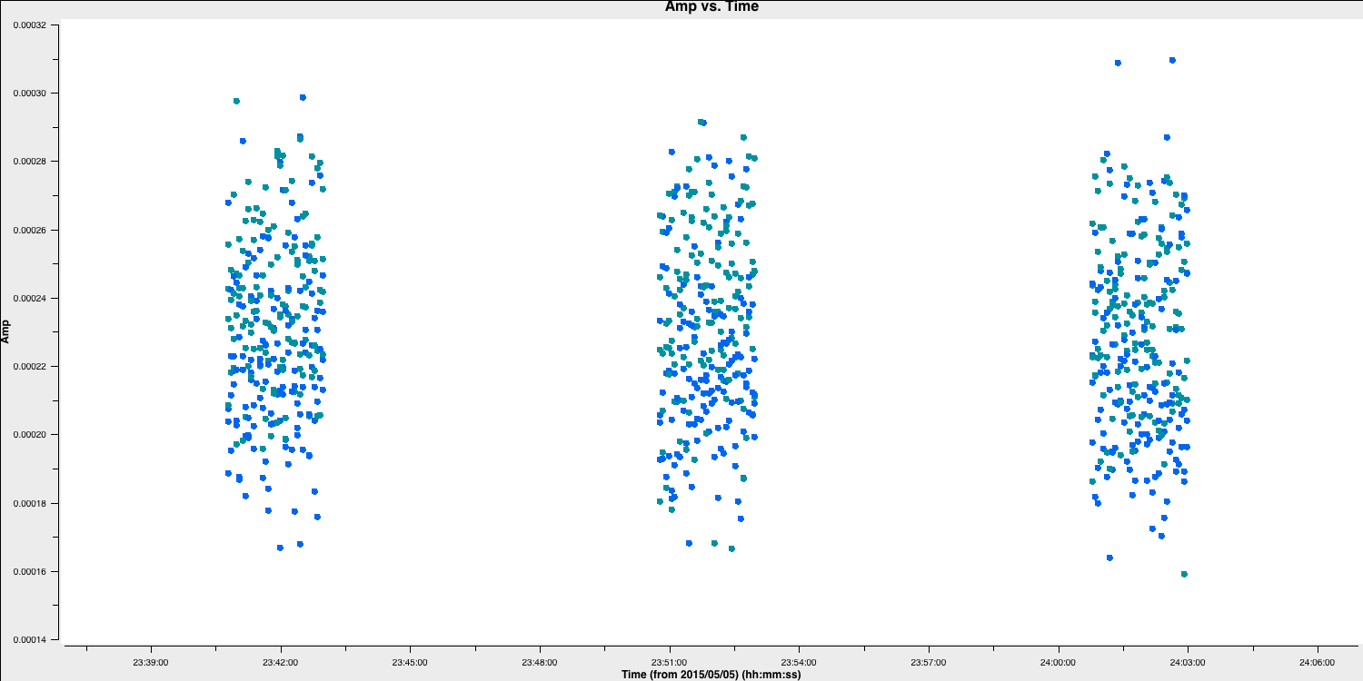
Roughly the same interval at the start of each scan is bad for all sources and antennas, so the phase reference is a good source to examine. (In a few cases there is extra bad data, ignore that for now). Use the Zoom and display to estimate the time interval (as is shown in the above plot, and we shall enter that value in next part.
2C. Flag the bad data at the start of each scan (step 3)
Remember from the EVN continuum tutorial that we need to always back-up our flags before we do any more flagging. This is so that we don't have to go back to the start in case we accidentally flag or un-flag large proportions of good data. We use flagmanager to do this.
	# Back up original flag state
	flagmanager(vis='***',
				mode='***',
				versionname='pre_quack')
If the parameters are set correctly, then we should have a backup named pre_quack in the all_avg.ms.flagversions file. You can check that it exists by running flagmanager again using mode='list' instead.
Next, we need to actually do the quacking or flagging of these channels. We use the CASA task flagdata to do this along with the special mode called quack. Fill in the flagdata parameters, inserting the time that the antennas were off source that we found earlier.
	# Flag first 40 s of each scan for all sources
	flagdata(vis='***',
			 mode='***', quackinterval='**')
Re-plot in plotms (tick reload option and replot if you still have it open) to check that the bad data at the start of each scan are gone. There are still some irregular periods of bad data which will be flagged later.
2D. Flag the bad end channels (step 4)
In this step, we are going to do the plotting and flagging all at once. To obtain the correct parameters for the flagging, it is advisable to copy and paste the plotms commands (with the correct parameters) into your CASA prompt and then input these parameters in the 3C277.1_cal_outline.py code for future reference.
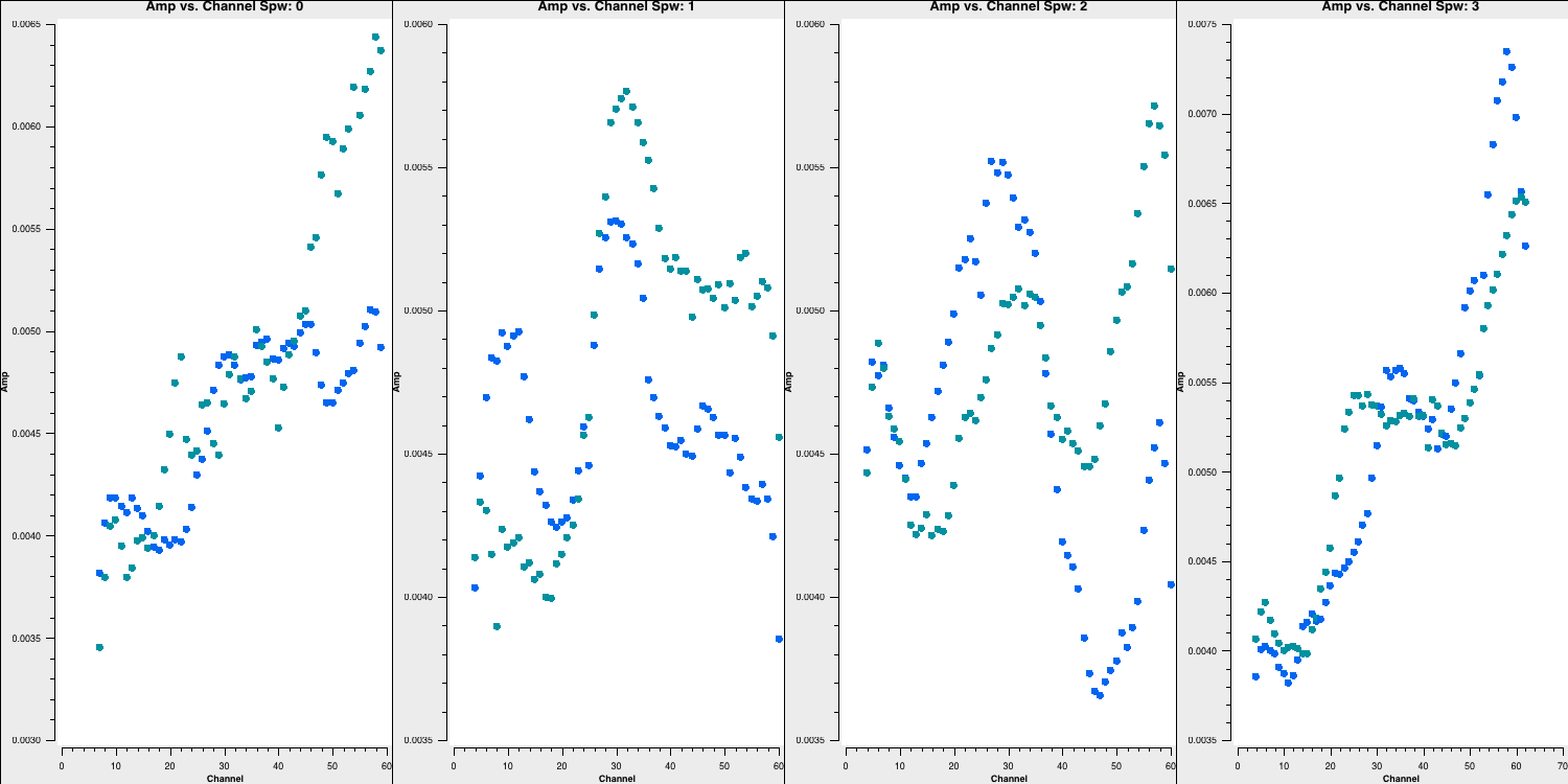
Let's continue. The edges of the bandpass for each spw are low sensitivity and must be flagged. This is the same for all sources, polarizations and antennas but different spectral windows may be different. Just look at the brightest source, 0319+415.
	plotms(vis='***',
		   field='***',
		   xaxis='***', yaxis='***', # plot amplitude against channel
		   antenna=***,             # select one baseline
		   correlation='**,**',     # just parallel hands
		   avgtime='***',           # set to a large number
		   avgscan=****,            # average all scans
		   iteraxis='***', coloraxis='***',  # view each spectral window in turn, and color
		   showgui=True,                     # change to False if you want ,
		   overwrite=True, plotfile='')
Take note of the channel ranges which are significantly less sensitive at each end of each spw.
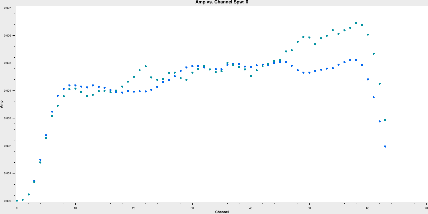
Back up the flags and enter the appropriate parameters in flagdata. Note the odd CASA notation for selecting spectral windows and channels. We have provided the "bad"/insensitive channels in spw 0 with the correct syntax, so use that as a guide for the other spectral windows.
	# Back up flags
	flagmanager(vis='***',
				mode='***',
				versionname='pre_endchans')

	# end chans
	flagdata(vis='***',mode='***',
			 spw='0:0~6;60~63,***')  # enter the ranges to be flagged for the other spw
Execute step 3 and then re-plot in plotms (the code should already do this replotting for you!)
2E. Identify and flag remaining bad data (step 5)
Finally, you usually have to go through all baselines, averaging channels and plotting amplitude against time. To save time (and sanity!), you don't have to do it all here. Have a look at 0319+419 and write down a few commands. This is done in the form of a list file, which has no commas and the only spaces must be a single space between each parameter for a given flagging command line. Some errors affect all the baselines to a given antenna; others (e.g. correlator problems) may only affect one baseline. Usually all spw will be affected so you can just inspect one but check afterwards that all are 'clean'. It can be hard to see what is good or bad for a faint target but if the phase-ref is bad for longer than a single scan then usually the target will be bad for the intervening time. Because the data are taken over two days, it is safest to use the full date for any time range.
Before we begin to flag, remember we should start by backing up the flags again!
	flagmanager(vis='all_avg.ms',
				mode='save',
				versionname='pre_timeflagging')
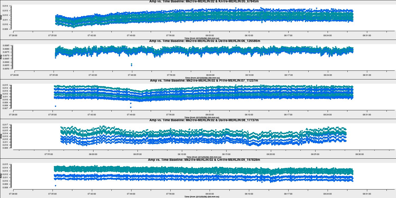
Use plotms to inspect 0319+415, plotting amplitude against time, RR,LL only, averaging all channels, all baselines to Mk2, paging (iterating) through the baselines.
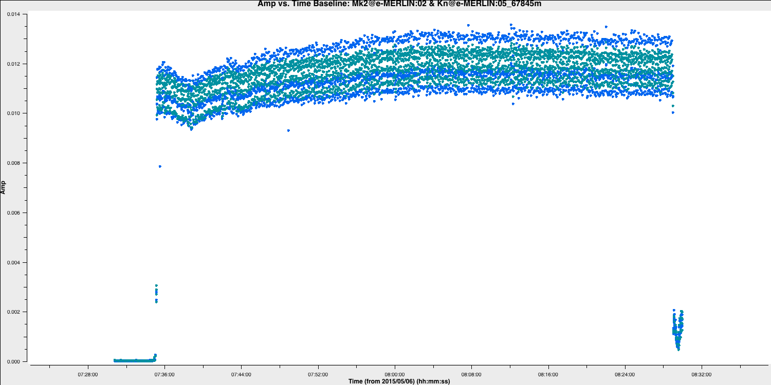
Here are some of the flagging commands in list format for the data shown below
mode='manual' field='0319+415' timerange='2015/05/06/07:30:00~07:35:00'
mode='manual' field='0319+415' antenna='Da' timerange='2015/05/06/07:30:00~07:56:22'
mode='manual' field='0319+415' antenna='Mk2&Kn' timerange='2015/05/06/07:30:00~07:35:34'
mode='manual' field='0319+415' antenna='Mk2&Kn' timerange='2015/05/06/07:48:55~07:48:58'
mode='manual' field='0319+415' antenna='Mk2,De' timerange='2015/05/06/07:35:00~07:35:18'
mode='manual' field='0319+415' timerange='2015/05/06/08:28:30~08:30:00'
Note that, by paging through all the baselines, you can figure out what bad data affect which antennas. Have a look at 1331+305 and write its commands.
The commands are applied in flagdata using mode='list', inpfile='***' where inpfile is the name of the flagging file. Write a file all_avg_1.flags with all the commands to flag bad data. Apply it in flagdata using mode='list'. Look carefully at the messages in the logger and terminal in case any syntax errors are reported.
Alternatively, if you are running out of time and don't want to flag, add instead all_avg.flags.txt as the inpfile command and it will flag all the data once you execute step 5.
Step 5 will also re-plot the data so check that it is now clean!
3. Calibration
3A. Delay calibration
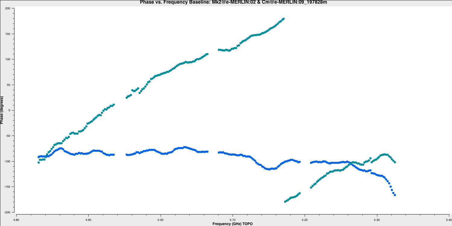
Begin by plotting the raw phase against frequency for a bright source. This is usually a bandpass calibrator.
	plotms(vis='all_avg.ms', field='0319+415', xaxis='frequency',
		   gridrows=1,gridcols=1,iteraxis='baseline', # Plot multiple baselines on one page
		   yaxis='phase',ydatacolumn='data',antenna=antref+'&*', # Plot all baselines to the reference antenna
		   avgtime='600',avgscan=True,correlation='LL,RR', # Average 10 min
		   coloraxis='corr',
		   plotfile='',
		   overwrite=True)
The y-axis spans -200 to +200 deg and some data has a slope of about a full 360 deg across the 512-MHz bandwidth. Looking at the baseline the Cambridge, think about the following questions.
QUESTION 1 What is the apparent delay error this corresponds to? What will be the effect on the amplitudes? Answer
A change of $2\pi$ radians in $x$ Hz results from a delay error of $1/x$ sec. So a change of 360 deg in 512 MHz is produced by a delay error of $1/(512\times 10^{6})\,\mathrm{sec} \sim 2\,\mathrm{ns}$. If data are vector-averaged across a phase slope, the amplitudes will be reduced, by a larger amount the greater the phase change in the averaging interval, so if the combined phase change on a baseline is worse in one polarisation than the other, that polarization will have a lower averaged apparent amplitude.
QUESTION 2 Delay corrections are calculated relative to a reference antenna which has its phase assumed to be zero, so the corrections factorised per other antenna include any correction due to the refant. Roughly what do you expect the magnitude of the Cm corrections to be? Do you expect the two hands of polarisation to have the same sign? Answer
The slopes on Mk2 correspond to about 1 turn in 512 MHz, in the same sense for both LL and RR. The slopes on Cm correspond to less than half a turn in the same sense for one polarisation, and about a full turn in the opposite sense for the other. So the combination of errors, which will be solved entirely by correcting Cm, corresponds to magnitudes of $\lesssim 1\,\mathrm{ns}$ and $\sim 4\,\mathrm{ns}$ for the two polarisations, with opposite signs. The slopes, and hence the actual values, vary between spw, see the delay correction plot.
Plot amplitude against time for just one channel per spw.
	# amp against time, longest baseline, single channel
	plotms(vis='all_avg.ms', field='0319+415',
		   spw='0~3:55', ydatacolumn='data',                     # Just one channel per spw
		   yaxis='amp', xaxis='time', plotrange=[-1,-1,0,0.018], # Plot amplitude v. time with fixed y scale
		   avgtime='60',correlation='RR', antenna=antref+'&Cm',  # 60-sec average, one baseline/pol
		   coloraxis='spw',plotfile='',
		   showgui=True,
		   overwrite=True)
Repeat with all channels averaged
	# amp against time, longest baseline, average all channels
	plotms(vis='all_avg.ms', field='0319+415',
		   xaxis='time', yaxis='amp',ydatacolumn='data',         # Plot amplitude v. time with fixed y scale
		   spw='0~3',avgchannel='64',                            # Average all unflagged channels
		   antenna=antref+'&Cm', avgtime='60',correlation='RR',  # 60-sec average, one baseline/pol
		   plotfile='',
		   plotrange=[-1,-1,0,0.018],coloraxis='spw',
		   showgui=True,
		   overwrite=True)
For the purposes of the same y axis scaling, these plots have been drawn in python. However, your plotms outputs should be semi-identical.
QUESTION 3 In the plots, which has the higher amplitudes - the channel-averaged data or the single channel? Why? Answer The single channel has the higher amplitudes. The source 3C84 is very bright so there is plenty of signal in each single channel. But averaging over all channels when there is a large phase slope causes the amplitudes to decorrelate so the channel-averaged data has depressed amplitudes. A similar effect is seen if you have data with phase errors as a function of time and average over too long a time period.
3A i. Derive delay corrections
The CASA task gaincal is used to derive most calibration. Type inp gaincal or help gaincal to find out more. Fill in the **.
	# Derive gain solutions
	os.system('rm -rf all_avg.K') # Remove any old version
	gaincal(vis='all_avg.ms',
			gaintype='**',            # Delay calibration (see help gaincal)
			field=calsources,         # All calibration sources
			caltable='all_avg.K',     # Output table containing corrections
			spw='0~3',solint='**',    # 600s solution interval
			refant=**,                # Reference antenna (phase set to 0)
			minblperant=2,            # For each antenna and solint, require solutions on
			minsnr=2)                 # at least 2 baselines with S/N > 2
Inspect the solutions. Are they of the magnitude you expect?
	plotms(vis='all_avg.K',
		   gridrows=2,
		   gridcols=3,
		   xaxis='**',
		   yaxis='**', # Plot delay against time
		   iteraxis='antenna', # Each antenna in a separate pane, coloured by spw
		   coloraxis='spw',
		   plotfile='all_avg.K.png')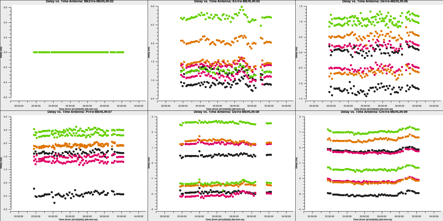
The solutions are stable in time, showing that the phase ref solutions can be applied to the target.
3B. Setting the flux of the primary flux scale calibrator (script step 7)
1331+305 (= 3C286) is an almost non-variable radio galaxy and its total flux density is very well known as a function of time and frequency (Perley & Butler 2013) . It is somewhat resolved by e-MERLIN, so we use a model made from a ~12-hr observation centred on 5.5 GHz. This is scaled to the current observing frequency range (around 5 GHz) using setjy which derives the appropriate total flux density, spectral index and curvature using parameters from Perley & Butler (2013).
However, a few percent of the flux is resolved-out by e-MERLIN; the simplest way (at present) to account for this is later to scale the fluxes derived for the other calibration sources by 0.938 (based on calculations for e-MERLIN by Fenech et al.).
The model is a set of clean components (see the imaging steps of the EVN continuum tutorial) and setjy enters these in the Measurement Set so that their Fourier transform can be used as a uv-plane model to compare later with the actual visibility amplitudes. If you make a mistake (e.g. set a model for the wrong source) use task delmod to remove it.
	setjy(vis='**',
		  field='**',
		  standard='Perley-Butler 2013',
		  model='**')  # You should have downloaded and untar'd this model
By default, setjy scales the model for each channel, as seen if you plot the model amplitudes against $uv$ distance, coloured by spectral window. If you have plotms running, go to the axes and select the model, or see the script for inputs. The model only appears for the baselines present for the short time interval for which 1331+305 was observed here. If not, then copy the following for plotms.
	os.system('rm -rf 3C286_model.png')
	plotms(vis='all_avg.ms', field='1331+305', xaxis='uvwave',
		   yaxis='amp', coloraxis='spw',ydatacolumn='model',
		   correlation='LL,RR',
		   showgui=True,
		   symbolsize=4, plotfile='')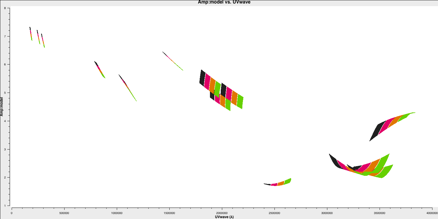
3C. Derive the initial bandpass calibration and inspect effects (script step 8)
For the next part we have a catch-22 situation (i.e. a paradoxical situation)!. In order to derive good time-dependent corrections, we need to average amplitude as well as phase in frequency, but in order to average in frequency we need the phase to be flat in time, and the amplitude to have the correct spectral index!
So we derive initial time-dependent solutions for the bandpass calibration sources, but discard these after they have been applied to derive the initial bandpass solutions. These, in turn, are replaced in script step 11.
3C i. Time-dependent pre-calibration to prepare for bandpass calibration
Estimate the time-averaging interval for phase by plotting phase against time for a single channel near the centre of the band for a bandpass calibration source. If the results for the first channel and antenna you try look bad, it may be a partly flagged channel; try a different one.
	plotms(vis='all_avg.ms',
		   field='**',    # Plot bandpass calibrator
		   spw='0~3:**', correlation='**'  # This gives all spw, choose channel in centre of spw in each and one correlation
		   antenna='**',  # Plot the longest baseline to the refant, likely to have the fastest-changing phase
		   xaxis='time', yaxis='phase',ydatacolumn='data', # Plot raw phase against time, no averaging
		   coloraxis='spw',plotfile='',
		   showgui=gui,
		   overwrite=True)
Zoom to help decide what phase solution interval to use. The integration-to-integration scatter is noise (mostly instrumental) which cannot be removed but the longer-term wiggles are mainly due to the atmosphere.
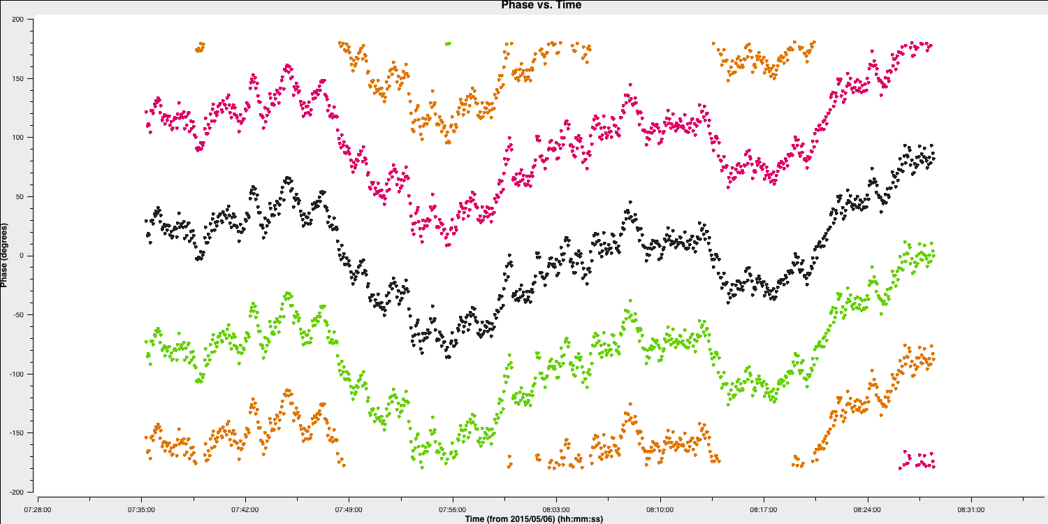
We want to derive corrections to reduce these to about the level of the noise or at least to less than 5-10 deg. The longer a solution interval, the better the S/N, but the interval has to be short enough not to average over the wiggles. To illustrate this, we have taken the phase fluctuations on spw 0, channel 55 and used different averaging intervals. This replicates the approximate solutions we would obtain when deriving the phases.
As you can see, the various solution intervals will track the long term slopes fairly effectively, however, the short 60s wiggles are only effectively tracked by the 30s solution interval. If we used the >60s intervals, we would still have errors ~20 deg whereeas, with the 30s intervals, the residuals will be nearer 5 deg.
QUESTION 4 What other effect, aside from atmospheric phase errors, is solved by calibrating phase against a point model at the phase centre? Answer The origin of phase is initially arbitrary, and different for each spw. The phase of a point source at the phase centre is flat at zero, so calibration should also line up all the phases close to zero, as well as taking out the wiggles.
Let's continue. Using the solution interval, which can track the wiggles, we want to derive the phase solutions using the task gaincal:
	os.system('rm -rf bpcals_precal.p1')
	gaincal(vis='all_avg.ms',
		    calmode='**',
		    field='**',
		    caltable='bpcals_precal.p1',
		    solint='**',
		    refant='**',
		    minblperant=2,
		    gaintable='all_avg.K',
		    minsnr=2)
Check the solutions. Each spw should have a coherent set of solutions, not just noise.
	plotms(vis='bpcals_precal.p1',
		   gridcols=3, gridrows=2,
		   xaxis='**',
		   yaxis='**',
		   plotrange=[-1,-1,-180,180],
		   iteraxis='antenna',
		   coloraxis='spw',
		   plotfile='bpcals_precal.p1.png')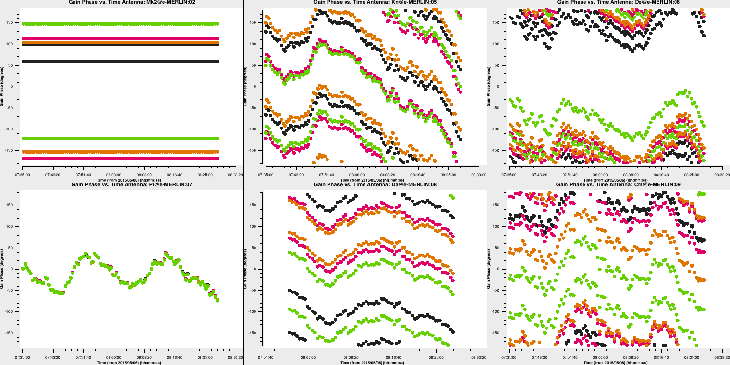
Note that the above plot is zoomed in on 0319+415 so we can see the phase solutions clearly. The plot of amplitude against time in Step 6 also showed that the uncorrected amplitudes have only a slow systematic slope with time, so a longer solution interval can be used, minimising phase noise.
QUESTION 5 Why solve for phase separately before solving for amplitude AnswerThe phase errors change on timescales of less than a minute, whilst the amplitude drifts more slowly with time. Applying phase solutions derived every 30-s, then allows the data to be averaged into longer solution intervals to improve the S/N when deriving amplitude solutions.
Now derive amplitude solutions. We have not yet derived flux densities for the bandpass calibration sources so we have to normalise the gains (i.e. individual solutions differ but the product is unity so that the overall flux scale is not affected). Thus we have to derive the solutions separately for each of the two bandpass calibrators, but write them to the same solution table.
	os.system('rm -rf bpcals_precal.ap1')
	gaincal(vis='all_avg.ms',
			field='0319+415',                # First bpcal
			caltable='bpcals_precal.ap1',    # Output solution table
			calmode='**',                     # Solve for amplitude and phase v. time
			solint='**',                     # Longer solution interval
			solnorm='**',                      # Normalise the amplitude solutions,
			refant='Mk2',
			minblperant=2,
			minsnr=2,
			append=False,
			gaintable=['all_avg.K','bpcals_precal.p1']) # Apply the existing delay and phase solutions

	gaincal(vis='all_avg.ms',
			field='1407+284',                # First bpcal
			caltable='bpcals_precal.ap1',    # Output solution table
			calmode='**',                     # Solve for amplitude and phase v. time
			solint='**',                     # Longer solution interval
			solnorm='**',                      # Normalise the amplitude solutions,
			refant='Mk2',
			minblperant=2,
			minsnr=2,
			append=True,
			gaintable=['all_avg.K','bpcals_precal.p1']) # Apply the existing delay and phase solutions
Alternatively, if are doing this in the CASA prompt, you can enter the parameters for the first source and then just adjust the field and append parameters.
Let's inspect the solutions in plotms:
	plotms(vis='bpcals_precal.ap1',
		   gridcols=3, gridrows=2,
		   xaxis='time',
		   yaxis='amp',
		   iteraxis='antenna',
		   coloraxis='spw',
		   plotfile='')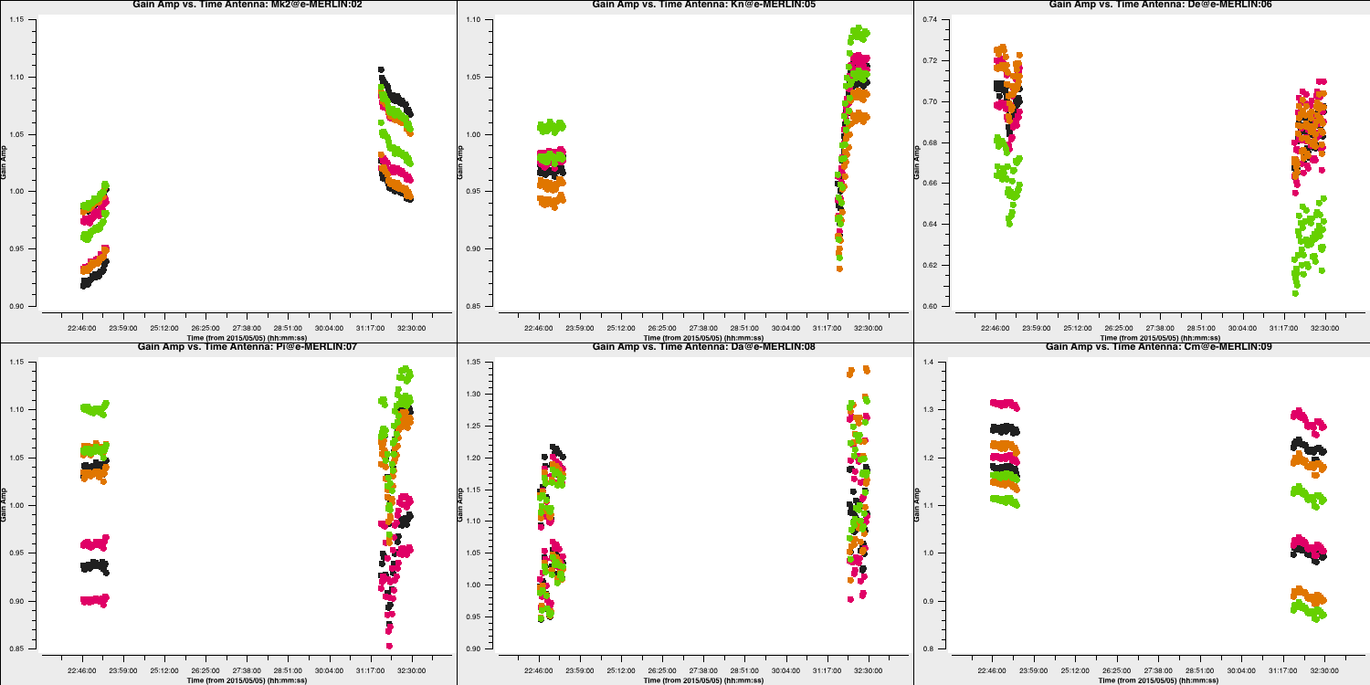
3C ii. Bandpass calibration
Use bandpass to derive solutions for phase and amplitude as a function of frequency (i.e., per channel). In order to allow averaging in time, apply the time-dependent corrections which you have just derived.
	os.system('rm -rf bpcal.B1')
	bandpass(vis='all_avg.ms',
			 caltable='bpcal.B1',         # New table with bandpass solutions
			 field='**,**',               # Bandpass calibration sources
			 fillgaps=16,                 # Interpolate over flagged channels
			 solint='inf',combine='scan', # Average the whole time for each source
			 solnorm='**',                # Normalise solutions
			 refant='**',
			 bandtype='B',
			 minblperant=2,
			 gaintable=['all_avg.K','bpcals_precal.p1','bpcals_precal.ap1'], # Apply all the tables derived for these sources
			 minsnr=3)
You may see messages about failed solutions but these should all be for the end channels which were flagged anyway.
Inspect the solutions in plotms. The phase corrections are small as the delay solutions were already applied. The amplitude solutions will remove local deviations from the bandpass but the corrections so far assume that the source flux density is flat in each spw.
Firstly, lets check phases:
	plotms(vis='bpcal.B1',
		   gridrows=2, gridcols=3,
		   xaxis='**', yaxis='**', # Plot phase solutions v. frequency
		   plotrange=[-1,-1,-180,180],
		   iteraxis='antenna',
		   coloraxis='spw',
		   plotfile='')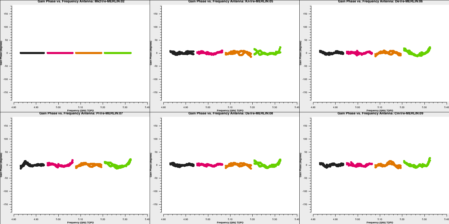
	plotms(vis='bpcal.B1',
		   gridrows=2, gridcols=3,
		   xaxis='**', yaxis='**', # Plot amp solutions v. frequency
		   iteraxis='antenna',
		   coloraxis='spw',
		   plotfile='')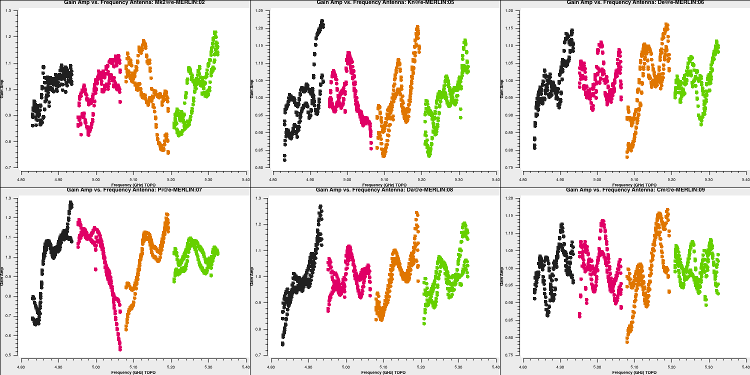
Apply the delay and bandpass solutions to the calibration sources as a test, to check that they have the desired effect of producing a flat bandpass for the phase-reference. There is no need to apply the time-dependent calibration as we have not derived this for the phase-reference source anyway.
Some notes about applycal:
- The first time
applycalis run, it creates theCORRECTEDdata column in the MS, which is quite slow. - Each time
applycalis run, it replaces the entries in theCORRECTEDcolumn, i.e. the corrected column is not cumulative, but you can giveapplycala cumulative list of gain tables. applymodecan be used to flag data with failed solutions but we do not want that here as this is just a test.- The
interpparameter can take two values for each gaintable to be applied, the first determining interpolation in time and the second in frequency. The times of data to be corrected may coincide with, or be bracketed by the times of calibration solutions, in which caselinearinterpolation can be used, the default, normally used if applying solutions derived from a source to itself, or from phase ref to target in alternating scans. However, if solutions are to be extrapolated in time from one source to another which are not interleaved, thennearestis used. A similar argument covers frequency. There are additional modes not used here (see helpapplycal).
The delay correction ('K') table contains entries for all sources except the target. The phase reference scans bracket the target scans so it is OK to use the default 'linear' interpolation.
The bandpass ('B1') table is derived from just two bandpass calibration observation and there may be data for other sources outside these times, so extrapolation in time is needed, using 'linear'. 'linear' interpolation is OK for the bandpass calibrator in frequency.
If you are finding your laptop is slow, you can skip this applycal and the plotms immediately after and just look at the figures here and go to Step 9.
	applycal(vis='all_avg.ms',
			 field='0319+415,1302+5748,1331+305,1407+284',
			 calwt=False,
			 applymode='calonly',   # Test, so don't change the weights or flag data with failed solutions
			 gaintable=['**','**'], # Enter the names of the tables used to calibrate the bandpass
			 interp=['**','**,**']) # The values depend on which table you listed first.
Check that the bandpass corrections are good for all data by plotting the 'before and after' phase reference phase and amplitude against frequency. First let's check the uncorrected phase (in the interactive CASA prompt this time!)
# In CASA:
default(plotms)
vis='all_avg.ms'; field='1302+5748'                 # Phase reference
xaxis='frequency';yaxis='phase';ydatacolumn='data'  # First, plot uncorrected phase
gridrows=5;gridcols=1;avgtime='600';coloraxis='scan'
iteraxis='baseline';antenna='Mk2&*';correlation='LL,RR'
plotms()
And next, the corrected phase,
ydatacolumn='corrected'
plotms()
Then, the uncorrected amplitude,
yaxis='amp'
ydatacolumn='data'
plotms()
And finally, the corrected amplitude,
ydatacolumn='corrected'
plotms()
The scripted versions of these commmands are also included in the 3C277.1_cal_outline.py script on lines 452-483. The plot below shows the uncorrected and corrected amplitudes and phases for the Mk2-Cm baseline of the phase reference source (1302+5748) that is coloured by scan. It has been replotted in python for clarity!
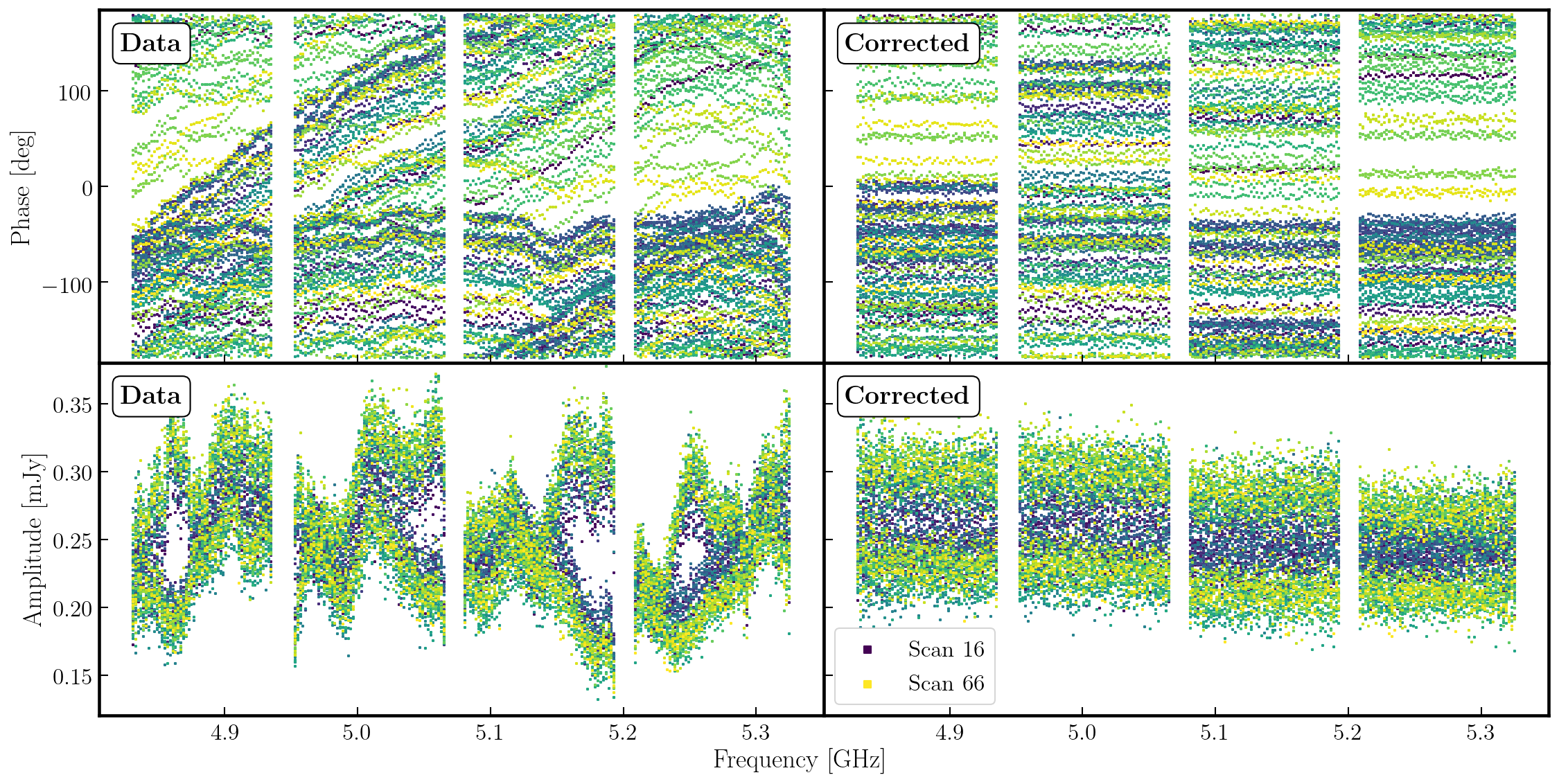
In the figure, each scan is coloured separately and shows a random offset in phase and some discrepancies in amplitude compared to other scans, but for each individual time interval it is quite flat. So we can average in frequency across each spw and plot the data to show remaining, time-dependent errors.
Plot the corrected phase against time with all channels averaged for the phase reference source. Zoom in on a few scans to deduce a suitable averaging timescale for correction of phase errors as a function of time, i.e. where atmospheric fluctuations dominate over noise. Again, we shall use the interactive CASA prompt.
# In CASA:
default(plotms)
vis='all_avg.ms'; field='1302+5748'
xaxis='time';yaxis='phase';ydatacolumn='corrected'
antenna='Mk2&*';iteraxis='baseline'
avgchannel='64'; coloraxis='spw'
correlation='LL'    # Just one pol as previous plots show both are similar
plotms()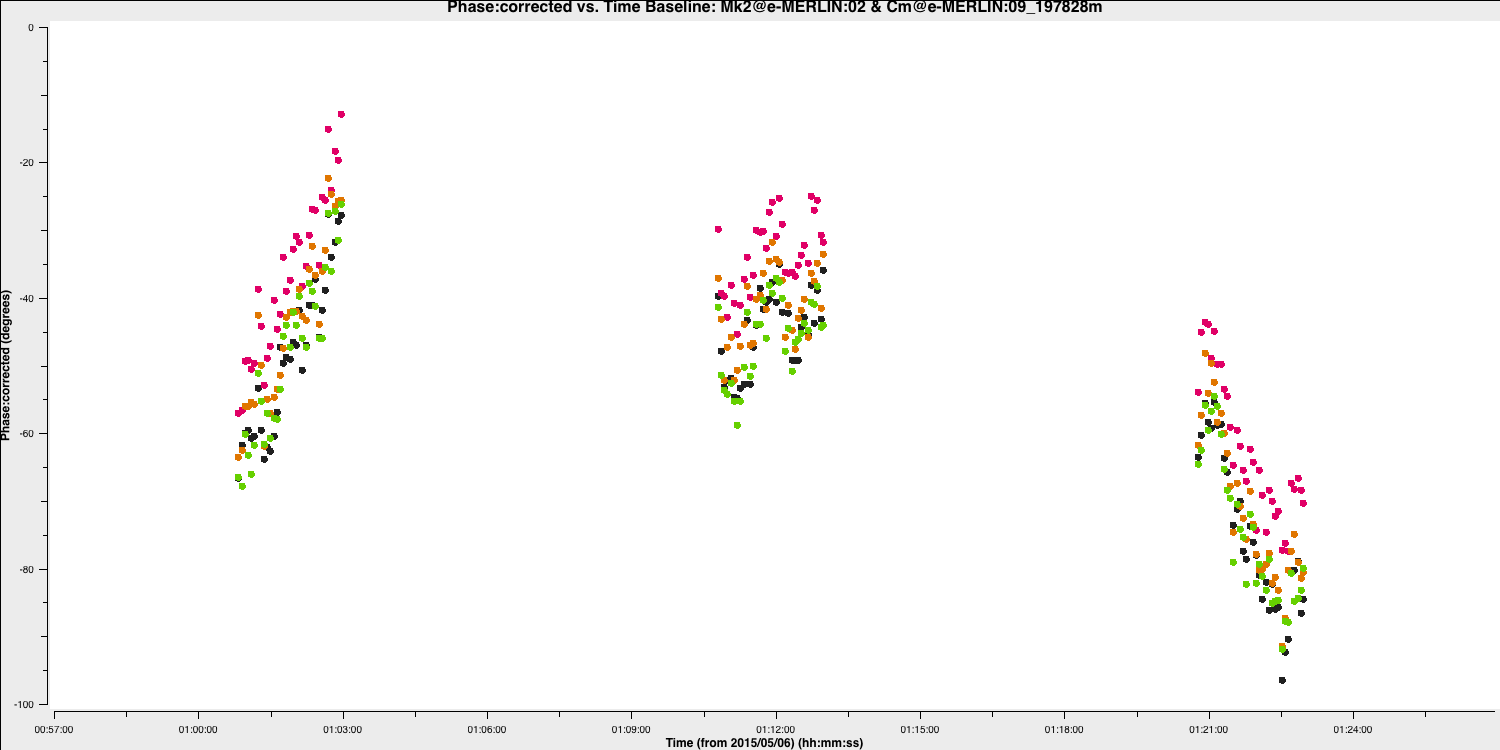
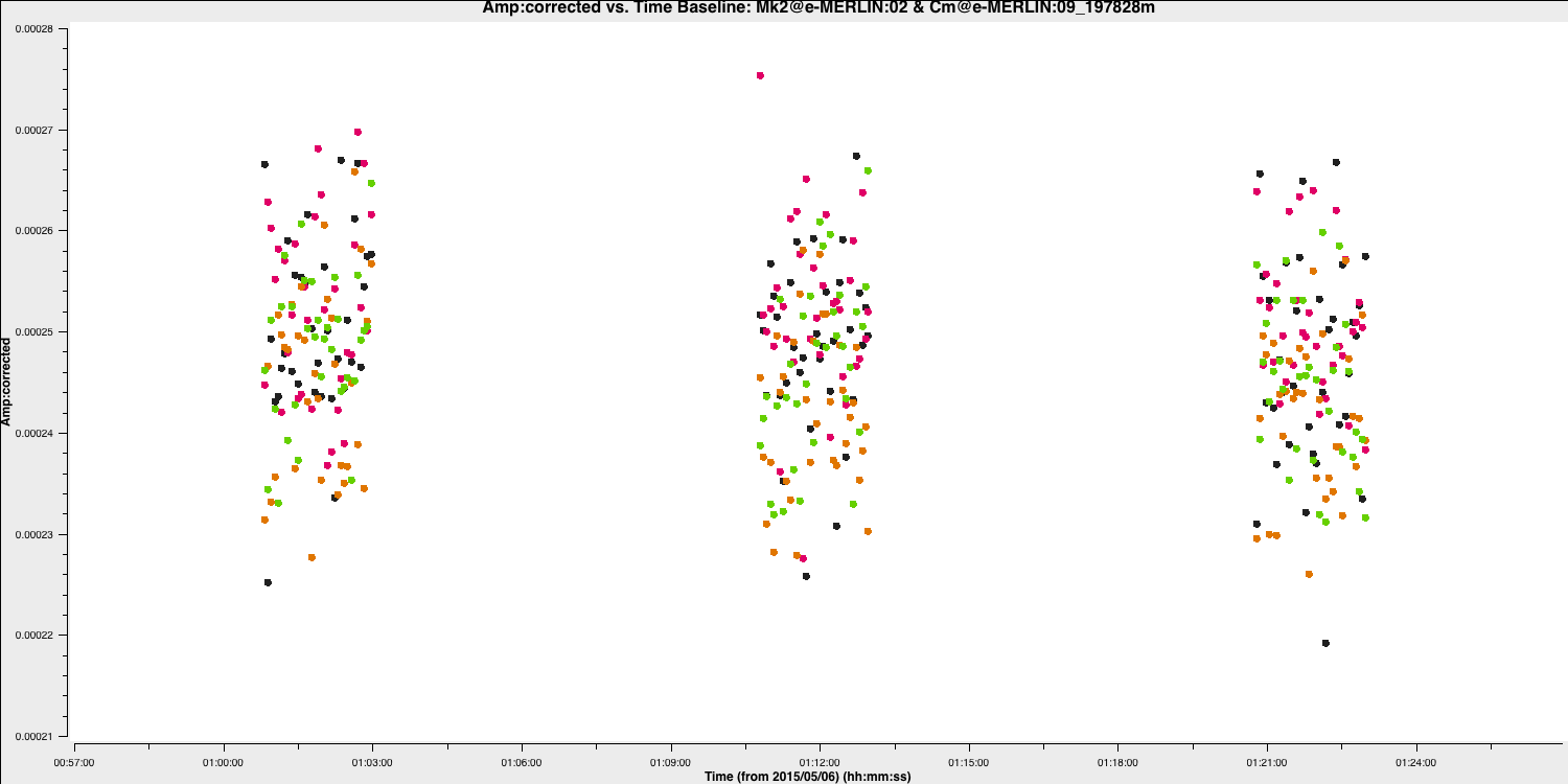
And repeat for amplitudes
3D. Gain calibration (script step 9)
3D i. Time-dependent phase calibration of all calibration sources
	gaincal(vis='all_avg.ms',
			calmode='p',              # Phase only first
			caltable='calsources.p1',
			field='**',               # All calibration sources
			solint='**',              # Insert solution interval
			refant=antref,
			minblperant=2,minsnr=2,
			gaintable=['all_avg.K','bpcal.B1'], # Existing correction tables to apply
			interp=['**','**,**'])              # Insert suitable interpolation modes
When you run gaincal, check the messages in the logger and the terminal. The logger shows something like:
2019-03-22 06:47:45	INFO		Writing solutions to table: calsources.p1
2019-03-22 06:47:46	INFO	calibrater::solve	Finished solving.
2019-03-22 06:47:46	INFO	gaincal::::	Calibration solve statistics per spw:  (expected/attempted/succeeded):
2019-03-22 06:47:46	INFO	gaincal::::	  Spw 0: 1400/935/930
2019-03-22 06:47:46	INFO	gaincal::::	  Spw 1: 1400/935/930
2019-03-22 06:47:46	INFO	gaincal::::	  Spw 2: 1400/935/930
2019-03-22 06:47:46	INFO	gaincal::::	  Spw 3: 1400/935/930
This means that although there are 1400 16s intervals in the calibration source data, about a third ($1400-935=465$) of them have been partly or totally flagged. But almost all ($99.4%$) of the intervals which do have enough unflagged ('attempted') data gave good solutions ('succeeded'). There are no further messages about completely flagged data but in the terminal you see a few messages when there are fewer than the requested 2 baselines per antenna unflagged:
Insufficient unflagged antennas to proceed with this solve.
(time=2015/05/06/06:32:26.5 field=0 spw=0 chan=0)
Here, there are very few, predictable failures. If there were many or unexpected failures, investigate - perhaps there are unflagged bad data, or pre-calibration has not been applied, or an inappropriate solution interval was used.
Plot the solutions, separately for L and R for clarity:
	plotms(vis='calsources.p1',
		   gridrows=2, gridcols=3,
		   xaxis='time',
		   yaxis='phase',
		   plotrange=[-1,-1,-180,180],
		   iteraxis='antenna',
		   coloraxis='spw',
		   correlation='L', # Note that solutions are per antenna, hence 'L' not 'LL'
		   plotfile='')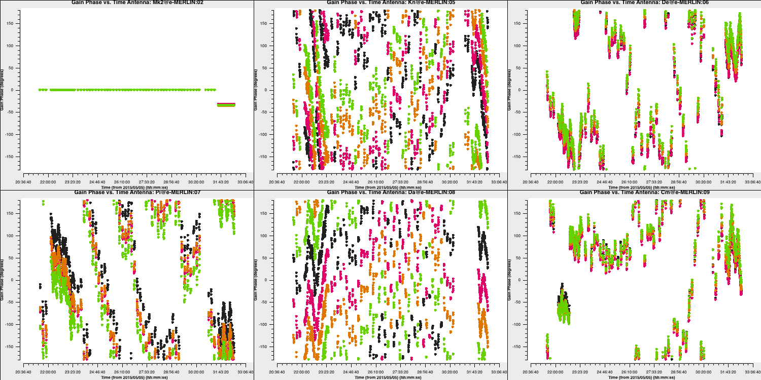
The phase corrections have a similar time-dependence as the uncorrected data phase, and are not random (if they look just like noise something is wrong).
3D ii. Time-dependent amplitude calibration of all calibration sources
Derive time-dependent solutions for all the calibration sources, applying the delay and bandpass tables and the time-dependent phase solution table.
At this point, 1331+305 has a realistic model set in the MS (Step 7). The other calibration sources have the default of a 1 Jy point source at the phase centre. If (and only if) you are repeating a failed attempt, reset any previous models for sources other than 1331+305.
# In CASA:
default(delmod)
vis='all_avg.ms'
field='0319+415,1407+284,1302+5748,1252+5634'
delmod()
Insert a suitable solution interval (from inspection of the previous amp plots and listobs output), the tables to apply and interpolation modes. Note that if you set a solint longer than a single scan on a source, the data will still only be averaged within each scan unless an additional 'combine' parameter is set, not needed here.
	gaincal(vis='all_avg.ms',
			calmode='ap',               # Amplitude and phase
			caltable='calsources.ap1',
			field='**',                 # All calibration sources
			solint='**',                # Insert solution interval.
			solnorm=False,              # Solutions will be used to determine the flux scale - don't normalise!
			refant='Mk2',
			minblperant=2,minsnr=2,
			gaintable=['all_avg.K','bpcal.B1','calsources.p1'],
			interp=['**','**,**','**']) # Insert suitable interpolation modes
The logger shows a similar proportion of expected:attempted solution intervals as for phase, but those with failed phase solutions are not attempted so all the attempted solutions work.
Plot the solutions separately for L and R for clarity:
	plotms(vis='calsources.ap1',
		   gridrows=2, gridcols=3,
		   xaxis='time',
		   yaxis='amp',
		   iteraxis='antenna',
		   coloraxis='spw',
		   correlation='L',
		   plotfile='')

	plotms(vis='calsources.ap1',
		   gridrows=2, gridcols=3,
		   xaxis='time',
		   yaxis='amp',
		   iteraxis='antenna',
		   coloraxis='spw',
		   correlation='R',
		   plotfile='')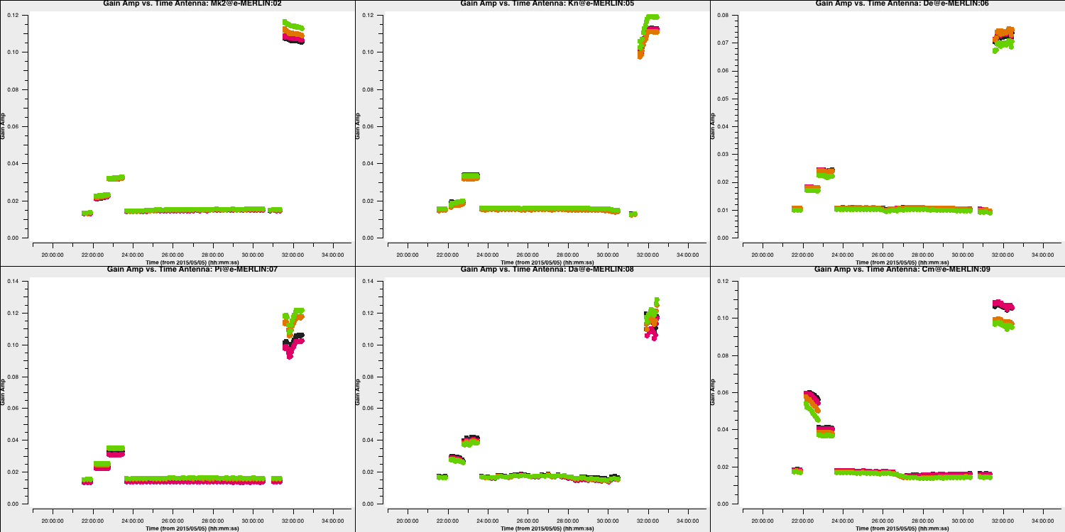
The plot above shows the time dependent amplitude solutions on just the L polarisation and coloured by spw. The solutions for each separate source look similar but there are big differences between sources, since they have all (apart from 1331+305) been compared with a 1 Jy model but they have different flux densities.
3E. Determining flux densities of calibration sources (script step 10)
3E i. Derive calibrator flux densities
The solutions for 1331+305 in calsources.ap1 contain the correct scaling factor to convert the raw units to Jy as well as removing time-dependent errors. This is used to calculate the scaling factor for the other calibration sources in the CASA task fluxscale. We run this task in a different way because the calculated fluxes are returned in the form of a python dictionary. They are also written to a text file. Only the best data are used to derive the flux densities but the output is valid for all antennas. This method assumes that all sources without starting models are points, so it cannot be used for an extended target.
	os.system('rm -rf calsources.ap1_flux calsources_flux.txt')
	calfluxes=fluxscale(vis='all_avg.ms',                # calfluxes will hold the calculated fluxes in memory
						caltable='calsources.ap1',       # Input table containing amplitude solutions
						fluxtable='calsources.ap1_flux', # Scaled output table
						listfile='calsources_flux.txt',  # Text file on disk listing the calculated fluxes
						gainthreshold=0.3,               # Exclude solutions >30% from mean
						antenna='!De',                   # Exclude least sensitive antenna
						reference='1331+305')            # Source with known flux density and previous model
If you type calfluxes this will show you the python dictionary, but if you don't yet know how to parse this, look at the logger or the listfile, calsources_flux.txt using:
!more calsources_flux.txt # Use of ! to invoke shell command
The individual spw estimates may have uncertainties up to $\sim20\%$ but the bottom lines give the fitted flux density and spectral index for all spw which should be accurate to a few percent. These require an additional scaling of $0.938$ to allow for the resolution of 1331+305 by e-MERLIN (see Setting the flux of the primary flux scale calibrator, step 7). The python dictionary calfluxes is used to do this:
	eMcalfluxes={}
	for k in calfluxes.keys():
		if len(calfluxes[k]) > 4:
			a=[]
			a.append(calfluxes[k]['fitFluxd']*0.938)
			a.append(calfluxes[k]['spidx'][0])
			a.append(calfluxes[k]['fitRefFreq'])
			eMcalfluxes[calfluxes[k]['fieldName']]=a
This makes a new python dictionary named eMcalfluxes, which we can print using print(eMcalfluxes) to produce:
{'1302+5748': [0.4043422839021926, -0.3654536785314739, 5069980155.629359],
 '1407+284': [1.9012873926908314, 0.30684493005193103, 5069980155.629359],
 '0319+415': [22.931908094424525, 1.3882373541791695, 5069980155.629359]}
where the first column or 'key' is the source name and the values are [flux density (Jy), spectral index and reference frequency (Hz)]. You may get slightly different values if you have chosen different solution intervals but if they are more than a few percent different something is probably wrong.
3E ii. Setting the calibrator flux densities
If you exit and restart CASA before running this step, you will have to re-define eMcalfluxes by copying the three lines starting with 'eMcalfluxes = ....' into the CASA prompt.
Nexe we shall use setjy in a loop to set each of the calibration source flux densities. The logger will report the values being set.
	for f in eMcalfluxes.keys(): # For each source in eMcalfluxes:
		setjy(vis='all_avg.ms',
			  field=f,
			  standard='manual',          # Use our values, not a built-in catalogue
			  fluxdensity=eMcalfluxes[f][0],
			  spix=eMcalfluxes[f][1],
			  reffreq=str(eMcalfluxes[f][2])+'Hz')
The default in setjy is to scale by the spectral index for each channel and plotting the models for the bandpass calibrators shows a slope corresponding to the spectral index (zoom in on the fainter source to see this). Both sources have positive spectral indices in this frequency range; this is less unusual for compact, bright QSO than for radio galaxies in general.
Plot the models for the bandpass calibrators, amplitude against frequency, to see the spectral slopes.
	plotms(vis='all_avg.ms', field='0319+415,1407+284',   # Plot the bandpass calibrators
		   xaxis='***',
		   yaxis='***',ydatacolumn='***',      # Fill in axis and data types
		   coloraxis='spw',correlation='LL',   # Just LL for speed; model is unpolarized
		   symbolsize=5, customsymbol=True,
		   symbolshape='circle',
		   plotfile='',overwrite=True)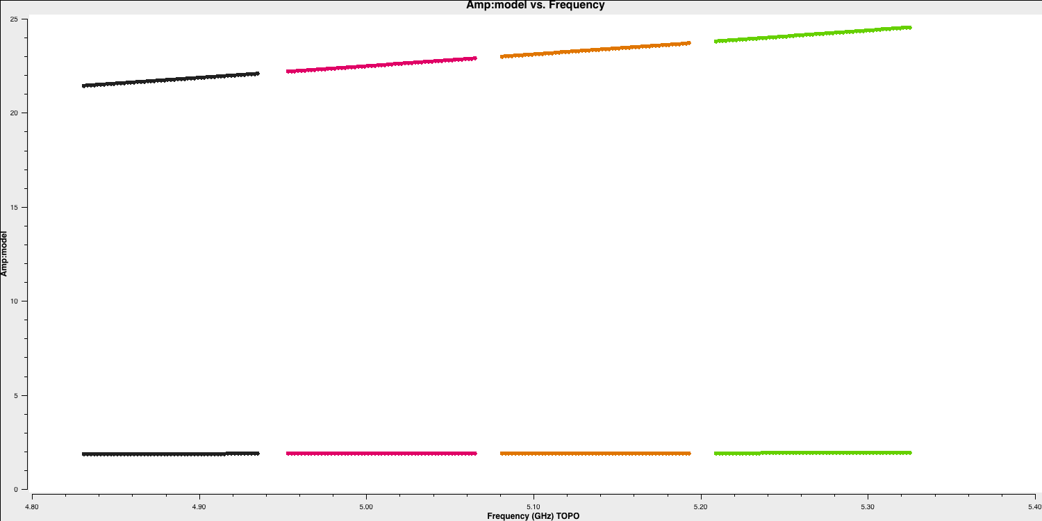
3F. Improved bandpass calibration (script step 11)
Use the models including spectral indices to derive a more accurate bandpass correction. You can use the first use of bandpass as a guide but there are three major differences (apart from writing a different table).
	os.system('rm -rf bpcal.B2')
	bandpass(vis='all_avg.ms',
		caltable='bpcal.B2',
		field='**,**',
		fillgaps=**,
		solint='**',combine='**',
		refant=antref,
		minblperant=2,
		solnorm='**',                      # There are now accurate flux densities and spectral indices so?
		gaintable=['all_avg.K','**','**'], # and updated time-dependent solutions
		gainfield='**,**',                 # but the new solutions contain entries for a number of sources
		minsnr=3)
And now we want to plot the solutions for both phase and amplitude:
	plotms(vis='bpcal.B2',
		   gridrows=2, gridcols=3,
		   xaxis='freq', yaxis='phase', # Plot phase solutions v. frequency
		   plotrange=[-1,-1,-180,180],
		   iteraxis='antenna',
		   coloraxis='spw',
		   plotfile='')

	plotms(vis='bpcal.B2',
		   gridrows=2, gridcols=3,
		   xaxis='freq', yaxis='amp', # Plot amp solutions v. frequency
		   iteraxis='antenna',
		   coloraxis='spw',
		   plotfile='')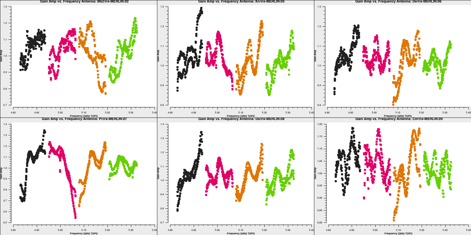
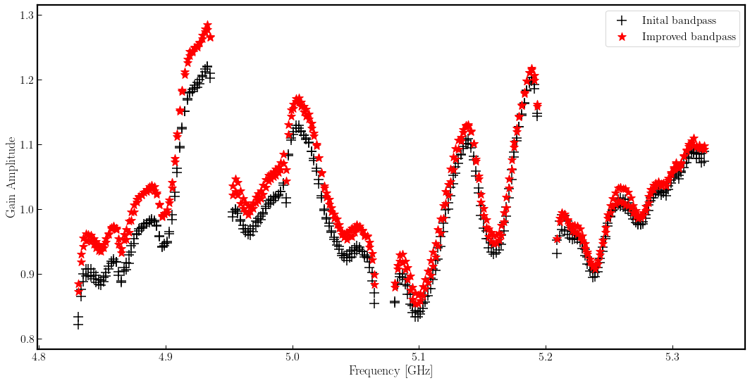
These solutions are similar to the initial bandpass approximation but with a different slope. To illustrate this, the initial bandpass and improved bandpass solutions for Knockin (Kn) are plotted below. You can see the same wiggles as in B1, but there is a different overall slope.
3G. Derive solutions for all cal sources with improved bandpass table (script step 12)
3G i. Derive amplitude solutions
For each calibration source, there is now a flux density and spectral index set for the MS MODEL column, as well as the delay, phase and improved bandpass calibration. These are used to derive time-dependent amplitude solutions which will both correct for short-term errors and contain an accurate flux scale factor.
Look at the previous time that you ran gaincal, and identify the one thing which you need to change now (apart from the output table name).
	os.system('rm -rf calsources.ap2')
	gaincal(vis='all_avg.ms',
			calmode='ap',
			caltable='calsources.ap2',
			field='**',
			solint='**',
			refant='**',
			minblperant='**',minsnr='**',
			gaintable=['**','**','**'],
			interp=['**','**,**','**'])
Plot the solutions:
plotms(vis='calsources.ap2',
		   gridrows=2, gridcols=3,
		   xaxis='time',
		   yaxis='amp',
		   iteraxis='antenna',
		   coloraxis='spw',
		   correlation='L',
		   plotrange=[-1,-1,0.01,0.06],
		   plotfile='') # repeat for other polarisation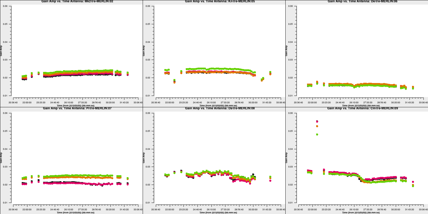
You expect to see a similar scaling factor for all sources. 1331+305 is somewhat resolved, giving slightly higher values for Cm (the antenna giving the longest baselines).
3G ii. Derive scan-averaged phase solutions to be applied to the target source
Finally, we need phase solutions that can be applied to the target source. Because we will interpolate solutions between phase calibrator scans, we just need one phase solution per phasecal scan. So solint should include all the data from each scan to form a solution.
	os.system('rm -rf calsources.p2')
	gaincal(vis='all_avg.ms',
			calmode='**',
			caltable='calsources.p2',
			field='**',
			solint='**',
			refant='**',
			minblperant=**,minsnr=**,
			gaintable=['**','**'],
			interp=['**','**,**'])
And again, we should plot the solutions:
	plotms(vis='calsources.p2',
		   gridrows=2, gridcols=3,
		   xaxis='time',
		   yaxis='phase',
		   iteraxis='antenna',
		   coloraxis='spw',
		   correlation='L',
		   plotrange=[-1,-1,-180,180],
		   plotfile='')
3H. Apply final calibrator source solutions and plot phase-ref and target (script step 13)
3H i. Apply solutions
Apply the bandpass correction to all sources. For the other gaintables, for each calibrator (field), the solutions for the same source (gainfield) are applied. gainfield='' for the bandpass table means apply solutions from all fields in that gaintable. applymode='calflag' will flag data with failed solutions which is ok as we know that these were due to bad data. We use the non-interactive format to allow us to use a loop over all calibration sources.
Cut and paste this all together; press return a few times afterwards till it runs.
cals = ['0319+415', '1302+5748', '1331+305', '1407+284']
for c in cals:
    applycal(vis='all_avg.ms',
             field=c,
             gainfield=[c, '',c,c],
             calwt=False,
             applymode='calflag',
             gaintable=['all_avg.K','bpcal.B2','calsources.p1','calsources.ap2'],
             interp=['linear','linear,linear','linear','linear'],
             flagbackup=False)                           # Don't back up flags multiple times here
Apply the phase-ref solutions to the target. We assume that the phase reference scans bracket the target scans so linear interpolation is used except for bandpass. Enter the parameters in interactive mode.
	applycal(vis='all_avg.ms',
			 field='1252+5634',
			 gainfield=['**','','**','**'], # Enter the field whose solutions are applied to the target
			 calwt=False,
			 applymode='**',  # Not too many failed solutions - OK to flag target data
			 gaintable=['**','**','**','**'],
			 interp=['**','**,**','**','**'],
			 flagbackup=True)
3H ii. Plot phase-ref and target amps against uv distance
Next we want to visualise our target and phase reference source. We want to ensure that the phase reference source is a true point source and if there is structure on the target. We can do this by looking at the amp vs uv distance plots. Remember a point source will be flat across uv distance!
	plotms(vis='all_avg.ms', field='1302+5748', xaxis='uvdist',
		   yaxis='amp',ydatacolumn='corrected',
		   avgchannel='64',correlation='LL,RR',
		   overwrite=True,
		   showgui=True,
		   coloraxis='spw')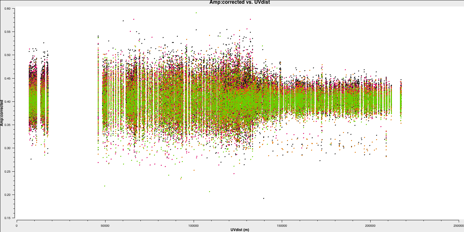
This looks pretty point-like!. Let's repeat the above for the target.
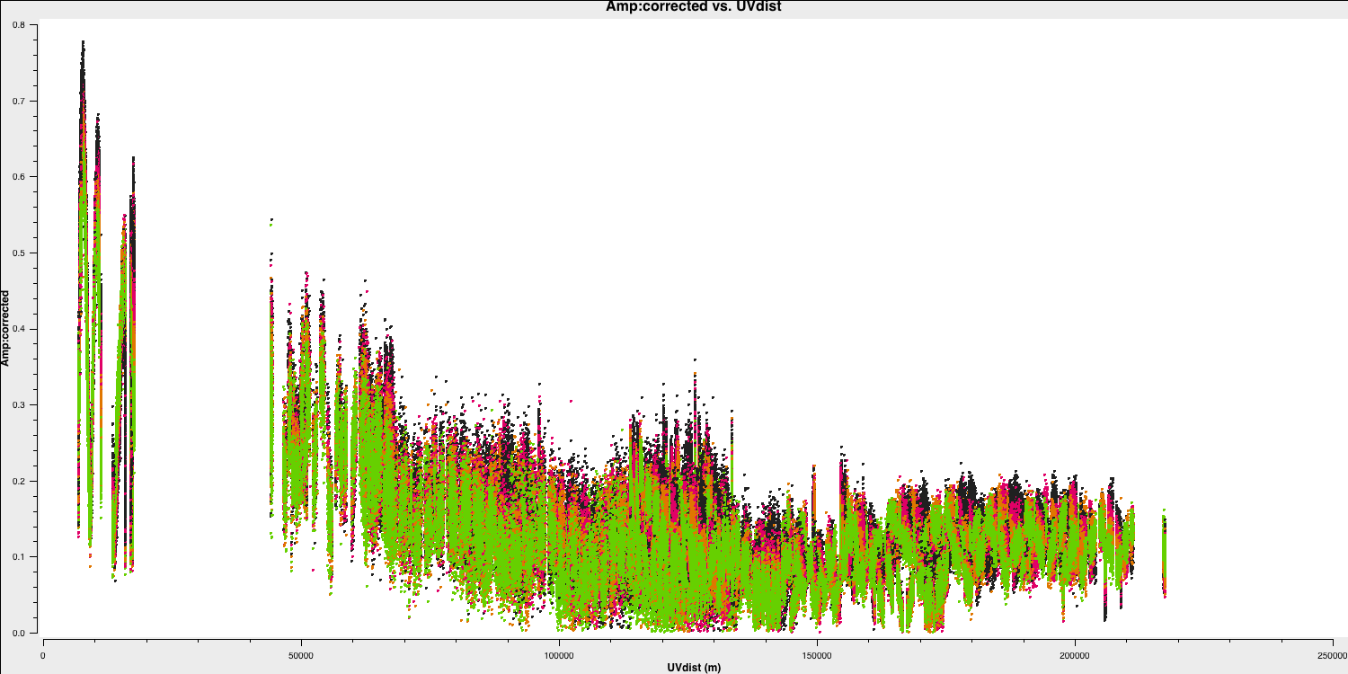
Hurray, there's some structure here!
As a test, QUESTION 6 What do the plots of amplitude against uv distance tell you? Answer
The visibility amplitudes for the phase ref are constant as a function of projected baseline length ($uv$ distance in metres), showing that it is point-like at e-MERLIN resolutions.
The amplitudes are noisiest out to 130km as these are the Defford baselines which are less sensitive. There's a little data which is anomalously low but this is ok as the target is bright.
The target has higher amplitudes on shorter baselines, showing that it has structure on scales larger than 50mas, and has complex structure on the long baselines.
3I. Split out target (script step 14)
Split out corrected target data. By default, this will take the corrected column.
	os.system('rm -rf 1252+5634.ms*')
	split(vis='all_avg.ms',
		  field='1252+5634',
		  outputvis='1252+5634.ms',
		  keepflags=True)
Now make sure that you save 1252+5634.ms for the imaging stages.
Script with solutions
If you had problems in any of the steps, you should use the calibration script 3C277.1_cal_all.py
Continue with imaging tutorial
You are ready to image the target source using the splitted calibrated data in 1252+5634.ms