
Part 3: Calibration & Imaging of 3C345
This section expects that you have completed parts 1 and 2 of the EVN continuum tutorial. You should now understand the basics of VLBI calibration and secondary calibration, including self-calibration and imaging. In this section, we will focus on our second pair of phase calibrator-target sources in this observation.
In the previous section, we merely input parameters into CASA tasks; this section expects you to generate a script independently with some guidance and pointers. It is structured to help you gain proficiency in applying these techniques to other data sets, and at the end, we will explore something new: weighting and analysing images.
Table of contents
- Data and supporting material
- How to approach this workshop
- Remove bad data
- Refining phase calibrator calibration
- Image phase calibrator
- Find phase calibration solution interval
- Correct residual delay & phase errors
- Apply phase calibration and re-image
- Generate amplitude solutions
- Apply corrections to phase cal
- Apply solutions to target and split
- Self-calibration on target
- Imaging the target
1. Data and supporting material
For this section, you will need the scripts contained in EVN_continuum_pt3_scripts_casa6.5.tar.gz (download link on the homepage) and the $uv$ data J1640+3946_3C345.ms from part 1. Place these two files into a separate folder so that you can distinguish between parts 1, 2, and 3 of this tutorial and un-tar the scripts. You should have the following in your folder:
J1640+3946_3C345.ms - Partially calibrated $uv$ data from part 1. If you encounter unusual results, please untar the NME_3C345_all.py- the complete calibration script in case you get stuck.NME_3C345_skeleton.py- the calibration script we will be inputting into.flag_TarPh.flagcmd- the complete flagging command list which removes residual bad data (only use if stuck or are low on time).flag_template.flagcmd- the template flagging commands for removing bad data.
EVN_continuum_pt3_uv_casa6.5.tar.gz file and use that measurement set.
2. How to approach this workshop
This workshop is a bit different from the previous parts and aims to assist you in generating a script from scratch. We will start by helping you with the task names; however, later on, this is entirely up to you (with some useful hints, of course!).
To begin:
- Open
NME_3C345_skeleton.py, and you will see that the preamble resembles the script from part 2.
The first thing we want to do is set some variables in the script to make it easier if you want to use the same script to reduce other similar data.
- Refer to lines 36-40 in the skeleton script and use the
listobstask to configure the parameters..
target='**' # target source
phscal='**'     # this is the phase calibrator
antref='**'     # refant as origin of phase
flag_table='**' # wait until step 2 to set this!
parallel=False  # Only works for linux atm (need to init with mpicasa -n <cores> casa)
You should have either remembered (from part 1) or identified that the phase calibrator is J1640+3946 and the target is 3C345. One thing you may have noticed from listobs is that there is a long scan of the target at the beginning of the observation. This is unusual, but we will recover this data.
- With these parameters set, examine the title of the steps and try to get a sense of the various actions we will take, while beginning to consider the CASA tasks we will use to achieve it.
If you are ready, we will begin filling in the script.
3. Remove bad data
3A. Inspect data
As you may remember, one of the best practices is knowing your data. This means inspecting it thoroughly and continuously during the calibration process. While in part 1, we removed the majority of bad data, the initial fringe fitting calibration has revealed some additional low-lying bad data. The first step we want to take is to identify the bad data and remove it.
- Refer to step 1 in the skeleton script and the provided hints. To identify bad data, use
plotmsto iterate over the various baselines and check for bad data (an example of bad data is shown below). - Include the
plotmscommands in step 1 of your code.
Instead of using the interactive flagging tool available in plotms, we aim to write a flag file to enable the same flagging if we need to restart from the beginning (as data can sometimes be lost or corrupted). Let's attempt to complete this.
- Open the file
flag_template.flagcmdwith your preferred text editor. - Review all the baselines again in
plotmsand use the search and locate function to identify the spw, field, baseline, and time range corresponding to the bad data. Record these in the flag file. - Remember to verify if this is limited to one baseline or applies to the entire antenna. This will decrease the number of flag commands you need to write in the file.
If you get stuck or want to compare the complete flag list, look at the flag_TarPh.flagcmd file. Note that if you are pressed for time, you can use this file to handle the flagging for you, as generating the flagging file can be time-consuming.
Once you are satisfied with your flag file, let's proceed to step 2, where we will apply the flags.
3B. Flag bad data
In this step, we will use our flagging commands to eliminate all the bad data and then verify that all the bad data has been removed.
- Refer to step 2 and include the parameters for the two tasks that should flag and then plot the cleaned data. Ensure that the flags are backed up in case the flagging process encounters issues. Use the
inp_fileparameter and set it to the name of the flagging file that you created. - If you are happy, execute step 2. If you find errors, review the syntax of your flag file and the indentation in your script.
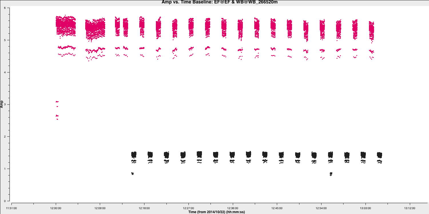
You should find that your data is clean. In the plot below, we illustrate this by showing the amplitude versus time for all baselines to the reference antenna. You can see that nearly all the bad data has been removed, and now we only have some mis-scaled amplitudes.
If you find that too much or too little data has been flagged, you should reset the flags using the restore function of the flagmanager task and select the version name you specified when saving the flags. You can then add or remove commands to your flag file and re-run step 2.
4. Refining phase calibrator calibration
If you recall from part 1, we encountered issues with the delays on Shenshen due to the instrumental delay jumps between scans. In part 2, we resolved this for the other phase calibrator-target pair by calculating delays and phase without combining the spectral windows. We will apply the same method here simply because our phase calibrator has sufficient flux to support this ($\sim 1.4\,\mathrm{Jy}$). Often, VLBI phase calibrators need to have all spectral windows combined to achieve enough S/N to derive accurate time-dependent delays, rates, and phases.
Now that the holding hands part is finished, no task names or parameters will be supplied from now on, putting calibration in your hands. However, not all is lost; the calibration steps are almost identical to those in part 2 of this workshop. Remember that you can refer to the NME_3C345_all.py file for the complete answers.
Best of luck, and let's keep going.
4A. Image phase calibrator
The first step we want to take is to image the phase calibrator to ensure that it is not resolved and, if it is, to provide a model to refine the delay and phase calibration. Remember, we also want to Fourier transform (FT) the model into the data for calibration purposes.
- Refer to step 3 and enter the two tasks that will image the phase calibrator, then Fourier transform the generated model into the measurement set.
- We want to track the S/N to monitor improvements at each calibration stage. The appropriate code is provided, so you only need to set the boxes again for the peak and r.m.s. values to be derived automatically.
You should find non-Gaussian noise, i.e., stripes around the phase calibrator, which are tell-tale signs of miscalibration. I managed to achieve a peak brightness, $S_p$, of $1.423\,\mathrm{Jy\,beam^{-1}}$, an r.m.s. of $0.027\,\mathrm{Jy\,beam^{-1}}$, resulting in a $\mathrm{S/N}= 52$. You should have values close to this.
4B. Find the phase calibration solution interval
The next step is to derive our phase calibration solution interval. Our phase calibrator and target are bright, so we should be able to track this on each baseline.
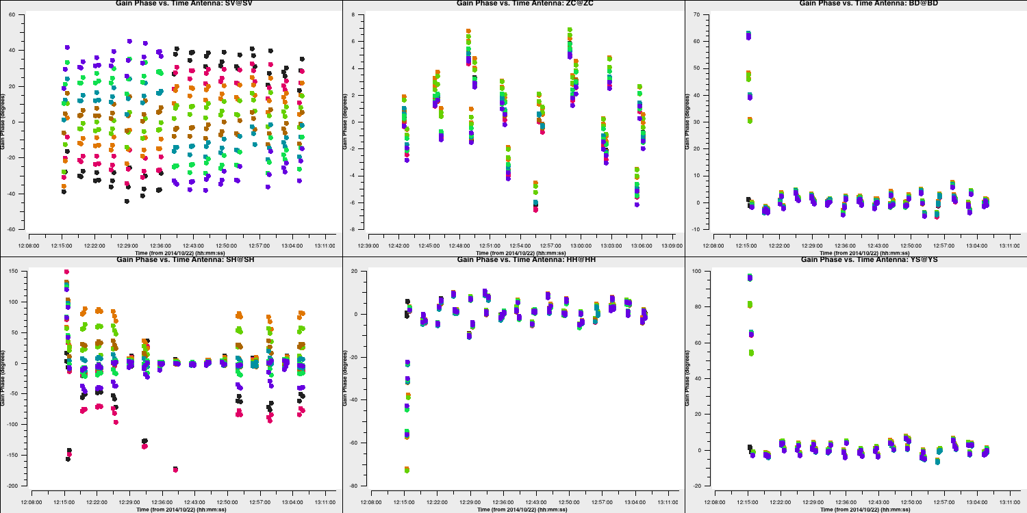
- In step 4, input the commands to plot the phase against time for the baselines relative to the reference antenna (which should be EF). We want to iterate over the baselines, so only one baseline should be plotted at a time. Additionally, ensure that the plot is colour-coded by field to differentiate between the target and phase calibrator easily.
- Execute the step, and you should get a plot similar to the one below.
- Iterate over the baselines and observe how all the phases are misaligned on the SH baselines. We will fix this in the next steps.
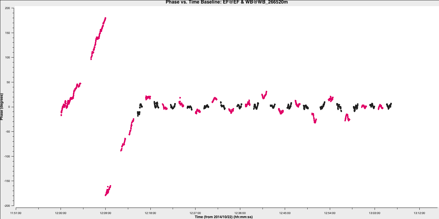
In particular, there are two factors about the above plot that are non-standard for radio interferometric observations, which you should keep in mind. This is a good exercise to familiarise yourself with your data. These are:
- We can track the target phases per baseline. Often, your target is not bright enough to achieve this and will appear more like uncalibrated noise. Note that the phases primarily follow the phase calibrator phases because we transferred our fringe-fitting solutions to the target in part 1 of this tutorial. However, you can observe that they deviate more than the phase calibrator scans. This is because the phase solutions on the phase calibrator are only approximately correct for the target field. These fluctuations are corrected using self-calibration on the target, as we did in part 2 for the other pair of sources.
- The target has long scans at the start of the observation, and their phases cannot be constrained due to the absence of surrounding phase calibrator scans. This situation is unusual because if the target was not bright enough for self-calibration, we wouldn't be able to self-calibrate these scans and would need to flag them. Otherwise, we would simply be adding noisy, uncalibrated data, leading to imaging errors. We will demonstrate the effect of including this uncalibrated data later.
Anyways, let's get back to it. If you remember from earlier, we want to track the phases within a scan, so we need at least two data points per scan. Determine which solution interval provides that, and remember it for the next section. Note that for delays, we want to maximize the S/N, so a per-scan solution interval should be sufficient.
4C. Correct residual delay & phase errors
Considering our solution intervals, we aim to derive the refined delay and phase solutions for our data.
- In step 5, type in the four tasks that will accomplish the following: 1) Produce delay calibration solutions per spw using a solution interval that maximises the S/N per scan. 2) Produce phase calibration solutions per spw using a solution interval that can track phases throughout the scan. 3) Plot both of these calibration tables, iterating over the antennas.
- Once you are satisfied, execute step 5, and you should obtain plots similar to those displayed below.
For delays:
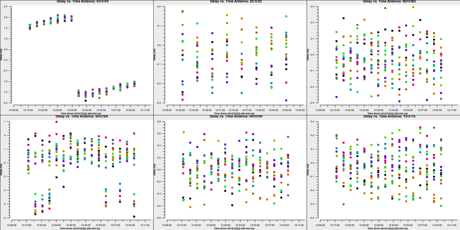
And for phases (using a 20 second solution interval):
You should notice that most solutions are small, as we have already obtained good ones through fringe fitting. However, the corrections on SH and SV are significant and should now suffice for calibrating this antenna.
4D. Apply phase calibration and re-image
The next step is to apply these solutions and re-image the phase calibrator again.
- In step 6, enter the four tasks that will accomplish the following:
- Apply the solutions we derived to the phase calibrator only. We want to ensure all calibrations are accurate before transferring to the target.
- Re-image the phase calibrator again (you can use parameters similar to those before, just ensure the image name matches the calibration steps so you can track it).
If you are using macOS, you must use the taskrun_icleaninstead oftclean. Due to bugs in the task, you need to explicitly set the parametersspecmode='mfs'andthreshold=0and do not set the parameterspsfcutofforinteractive. - Fourier transform the model into the phase calibrator visibilities.
- Extract the peak flux and r.m.s. from the generated image to determine the S/N.
- Once you are happy, then execute step 6.
I achieved a modest improvement with $S_p = 1.493\,\mathrm{Jy\,beam^{-1}}$, $\sigma= 0.028\,\mathrm{Jy\,beam^{-1}}$ and so a $\mathrm{S/N}=54$
4E. Generate amplitude solutions
Next, we want to derive amplitude solutions since we observed some mis-scaled amplitudes during the flagging step. This should align all of our antennas and significantly increase our S/N.
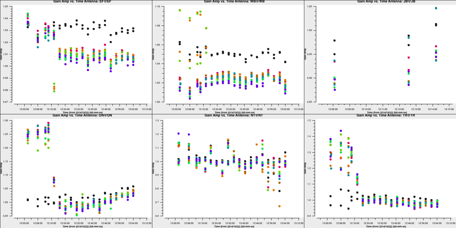
- In step 7, input the task that will produce amplitude solutions. We want to maximise the S/N for amplitudes (which typically vary more slowly with time), so you should use a longer solution interval. Usually, a per-scan interval will suffice. Keep in mind that we have already set the flux scaling, so we want the solutions to be normalised to avoid changing this. Additionally, remember that we need to apply all previous calibration on the fly in this task.
- Also include the task of plotting these solutions per antenna to ensure that the solutions are sensible.
You should find corrections that are similar to those shown below:
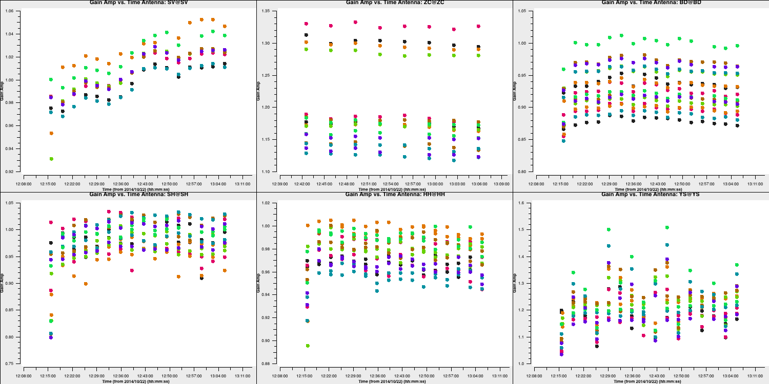
Some antennas have re-scaling applied, but most solutions are close to unity. The first scan has some rescaling applied and also had significant corrections in the phase solutions. Let's verify the calibration by imaging again.
4F. Apply corrections to phase cal
Next, we need to apply the amplitude solutions to the phase calibration and evaluate these solutions by imaging the phase calibrator one final time.
- IIn step 8, input the tasks that will apply all of the calibration derived so far to the phase calibrator. Remember, CASA calibration always applies corrections to the original $\texttt{DATA}$ column, not the $\texttt{CORRECTED}$ data, so all calibration needs to be applied again.
- In this step, image the phase calibrator once more and evaluate the improvements by calculating the S/N as previously.
- A total of three different tasks should be used for this. Note that we no longer need to FT the model into the visibilities, as calibration on the phase calibrator is complete.
The resulting image should demonstrate a dramatic increase in the S/N, and the non-Gaussian ripples should have significantly reduced in amplitude. I obtained $S_p = 1.563\,\mathrm{Jy\,beam^{-1}}$, $\sigma= 1.37\,\mathrm{mJy\,beam^{-1}}$ and so a $\mathrm{S/N}=1138$. You should aim for a similar S/N (at least 500 or higher).
4G. Apply solutions to target and split
Since we are pleased with the calibration refinements we made, we should now apply these to our target source.
- In step 9, enter the command that will apply the calibration solutions to the target source. Keep in mind that we want to linearly interpolate these onto the target, as the scans are interleaved with the phase calibrator scans.
- Input the command that will subsequently extract the corrected target data into a separate measurement set named
3C345.ms. This will now serve as our new data set for the self-calibration of the target field.
5. Self-calibration on target
In the next steps, we will focus exclusively on the target source. Our phase calibrator should have provided us with the approximately correct phase versus time and frequency. However, we aim to refine this and eliminate the phase differences induced by the atmospheric variations between the phase calibrator and the target fields. We will use self-calibration to achieve this.
5A. First image of target
The first step we want to take for self-calibration is to create a good model of our source.
- In step 10, enter the commands to generate an image of the target source. Remember that we should be working from the new measurement set that we have just created.
- Input the commands to measure the S/N ratio.
We should remember something from before: the long scan of the target that remained uncalibrated after the phase referencing. By including these scans, you'll find that your S/N of the initial target is $\leq10$ (I got $S_p = 1.614\,\mathrm{Jy\,beam^{-1}}$, $\sigma = 0.174\,\mathrm{Jy\,beam^{-1}}$ and a $\mathrm{S/N=9}$). Let's see what happens when we exclude this data.
- In step 10, configure the
timerangeparameter in the imaging task to exclude the uncalibrated portions of the data. - Complete step 10, but remember to either change the image name or remove the first set of images created beforehand; otherwise, it will crash!
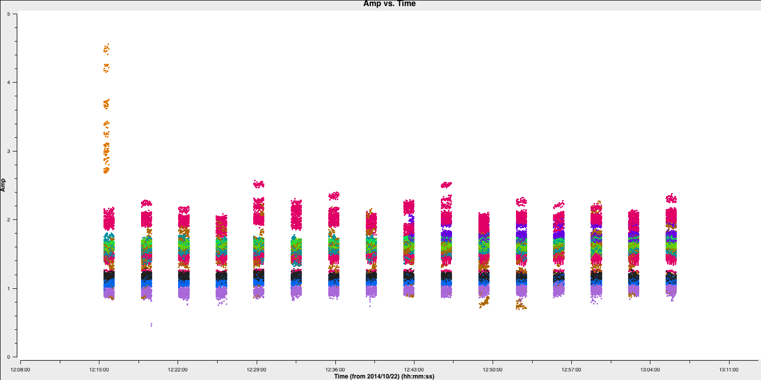
By excluding these scans, you should observe a dramatic increase in the S/N. I obtained $S_p = 2.453\,\mathrm{Jy\,beam^{-1}}$, $\sigma = 0.029\,\mathrm{Jy\,beam^{-1}}$ and a $\mathrm{S/N=84}$. The plot below illustrates this. You can see the various amplitude and phase errors in the left panel (deep troughs), where the uncalibrated data is included, while the right panel is much cleaner and exhibits a higher peak flux density. Note that the color scale is identical for both plots.
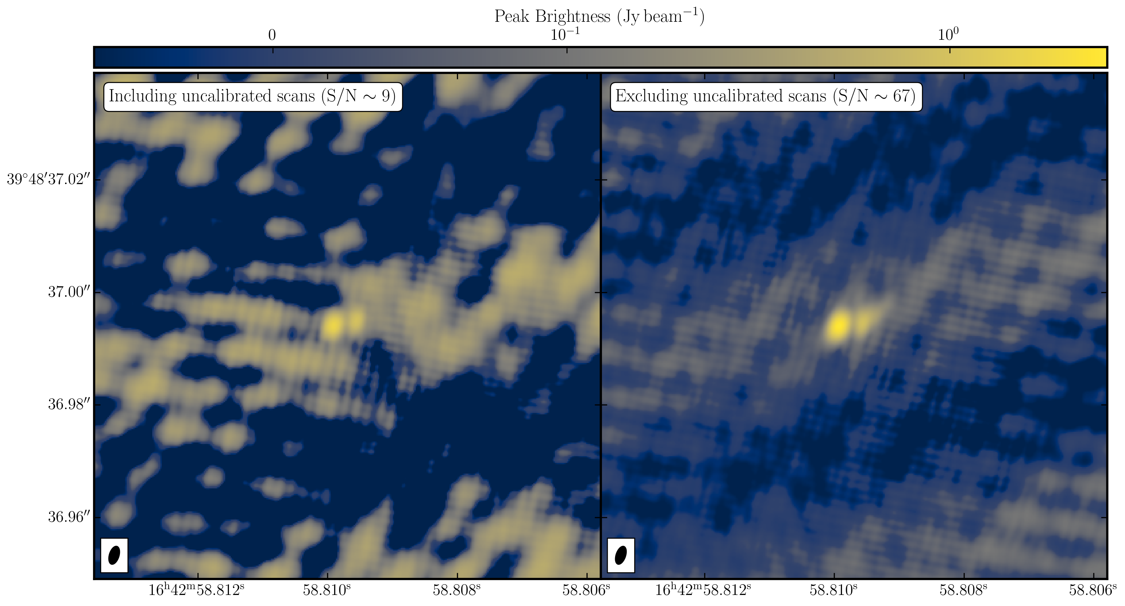
This is a prime example of understanding your data and highlights how retaining 'bad' or uncalibrated data can negatively impact your radio images. This is why understanding your data, devising a calibration strategy, and eliminating RFI can significantly enhance your calibration of radio interferometric data.
In this case, we need to decide what we are going to do with these uncalibrated scans. We could either: 1) flag the data or 2) attempt to calibrate it. Flagging the data would be simple; however, we would sacrifice sensitivity as a consequence. Instead, we can try using the model derived from the calibrated scans to calibrate the uncalibrated long scans. A signal-to-noise ratio of greater than 50 should be sufficient to achieve this.
5B. Self-calibration phase
Let's remove the atmospheric phase fluctuations on the target field and calibrate the initial scans. Additionally, we need to consider a suitable solution interval to track the phase within a scan!
- In step 11, type in the task to derive phase only calibration solutions and plot these solutions for each antenna. Remember that to track phases within scans, we want at least two points per scan, so adjust your solution interval accordingly.
- If you feel happy, run step 11.
If everything went according to plan (and the correct model is FT with the data, i.e., without the uncalibrated scans), you should obtain phase solutions similar to those below:
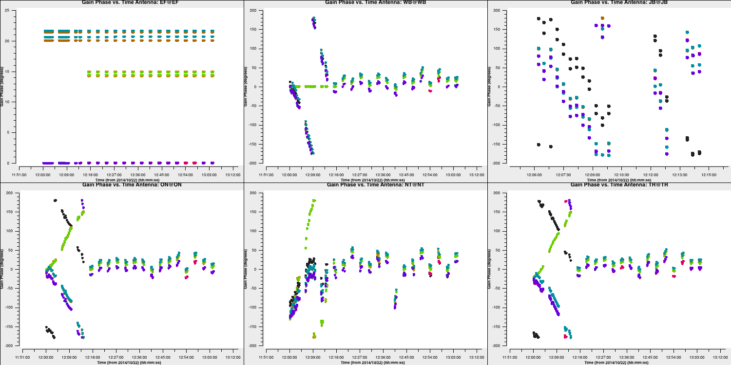
Hooray! Our calibration strategy seems to have worked, as the initial uncalibrated scans display phase corrections that are broadly similar to the phase versus time plots we created in part 4B of this tutorial. For the remaining scans, the corrections are minor (approximately $ 30^\circ$), but they should correct for the atmospheric differences between the target and the phase calibrator.
- Let us proceed to step 12. Now that we have solutions, we need to apply them to the data to generate the $\texttt{CORRECTED}$ data column. The type of interpolation is important here.
- In this step, we also want to image the target again and track the improvements in S/N we obtained from our calibration.
- Additionally, this new model should undergo Fourier transformation into the measurement set to update the model column for further self-calibration.
- You'll need five tasks for this part, and once you're satisfied with your entries, execute step 12.
I achieved a slight increase in S/N to 98 ($S_p = 2.700\,\mathrm{Jy\,beam^{-1}}$, $\sigma = 0.028\,\mathrm{Jy\,beam^{-1}}$). This is primarily due to the increase in peak flux density. The phases determine where the flux density is; therefore, miscalibrated phases shift a portion of flux from the source into the noise. Recalibrating this can thus increase the peak flux density while simultaneously reducing the noise.
5C. Amplitude self-calibration
In the previous section, we carried out a self-calibration cycle to correct for phases. Our next task is to correct for amplitude errors. Most of these errors, arising from the antennas, should have been addressed by the amplitude calibration on the phase calibrator. However, some scan-to-scan differences may still need correction.
- In step 13, enter the task to derive amplitude and phase calibration solutions and plot these solutions for each antenna. Remember that for amplitudes, one point per scan is often sufficient, as we want to maximise signal-to-noise ratio (S/N).
- If you are happy, execute step 13.
You should find some slight adjustments, particularly in the first, previously uncalibrated scan, which should resemble the plot below:
Next, we should look to see if the amplitude self-calibration has improved our target image.
- In step 14, include the tasks that will 1) apply the calibration solutions, 2) image the calibrated data, and 3) track the S/N increase. This should consist of three tasks.
- Execute step 14.
You should see a significant improvement in the S/N to 876 ($S_p = 2.736\,\mathrm{Jy\,beam^{-1}}$, $\sigma = 3.123\,\mathrm{mJy\,beam^{-1}}$).This is primarily because the initial scan is now fully calibrated.
Next, we want to visualise the data in different ways to investigate the structure of the source.
For bookkeeping purposes, we should separate the fully calibrated data. This has already been provided in step 15, so:
- Execute step 15 to produce
3C345_calibrated.ms.
6. Imaging the target
6A. Optimising sensitivity via reweighing
Since we have a heterogeneous array, the optimal weights when imaging should consider the sensitivities of the baselines; that is, more sensitive baselines receive higher weights. Calibration can facilitate this process, but the best approach is to examine the noise on each baseline to estimate the sensitivity. More sensitive baselines will exhibit less noise.
Fortunately, CASA includes a task called statwt that performs this function. It estimates the standard deviation of the noise on each baseline and readjusts the weights accordingly. This task must be executed after calibration, as miscalibrated data or RFI can negatively impact the weight estimation.
- Refer to step 16. The
statwtcommand has been entered for you. We will use the default parameters and estimate the weights from the $\texttt{DATA}$ column since we are now using the split dataset. - We want to examine the weights assigned, so input the parameters into
plotms, which will plot the weight versus the uv wave for all baselines to Onsala. This should create a plot similar to the one below (colored by baseline).
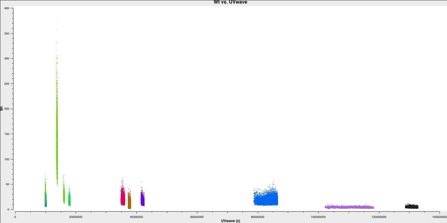
As you can see, the highest weight is given to the baselines with the largest telescope (i.e., Effelsberg). This means that these baselines will be emphasised more in imaging, resulting in optimal sensitivity.
6B. Experimenting with weighting
For the final part of this workshop, we will experiment with adjusting the weighting during imaging. From the lectures, you may know that the weighting applied to the data influences the spatial scales represented in the imagery. This is important because changing the weighting often reveals more structure.
- Refer to step 17 and input the parameters into
tclean/run_iclean, which will generate three images with natural, uniform, and robust (0.5) weightings. - You may need to decrease the cell size for the uniform weighted image.
- Clean the images and then look at them in the viewer/CARTA.
The naturally weighted image should offer the best sensitivity, though with poorer resolution. This occurs because the more sensitive, yet shorter, central European baselines dominate the weights, resulting in lower resolution.
In contrast, the uniformly weighted image increases the weighting of longer baselines, which improves the resolution and reveals a more complex structure of the source. In particular, the left blob now has two components. However, this increase in resolution comes at the cost of reduced sensitivity, as the sensitive European baselines are down-weighted.
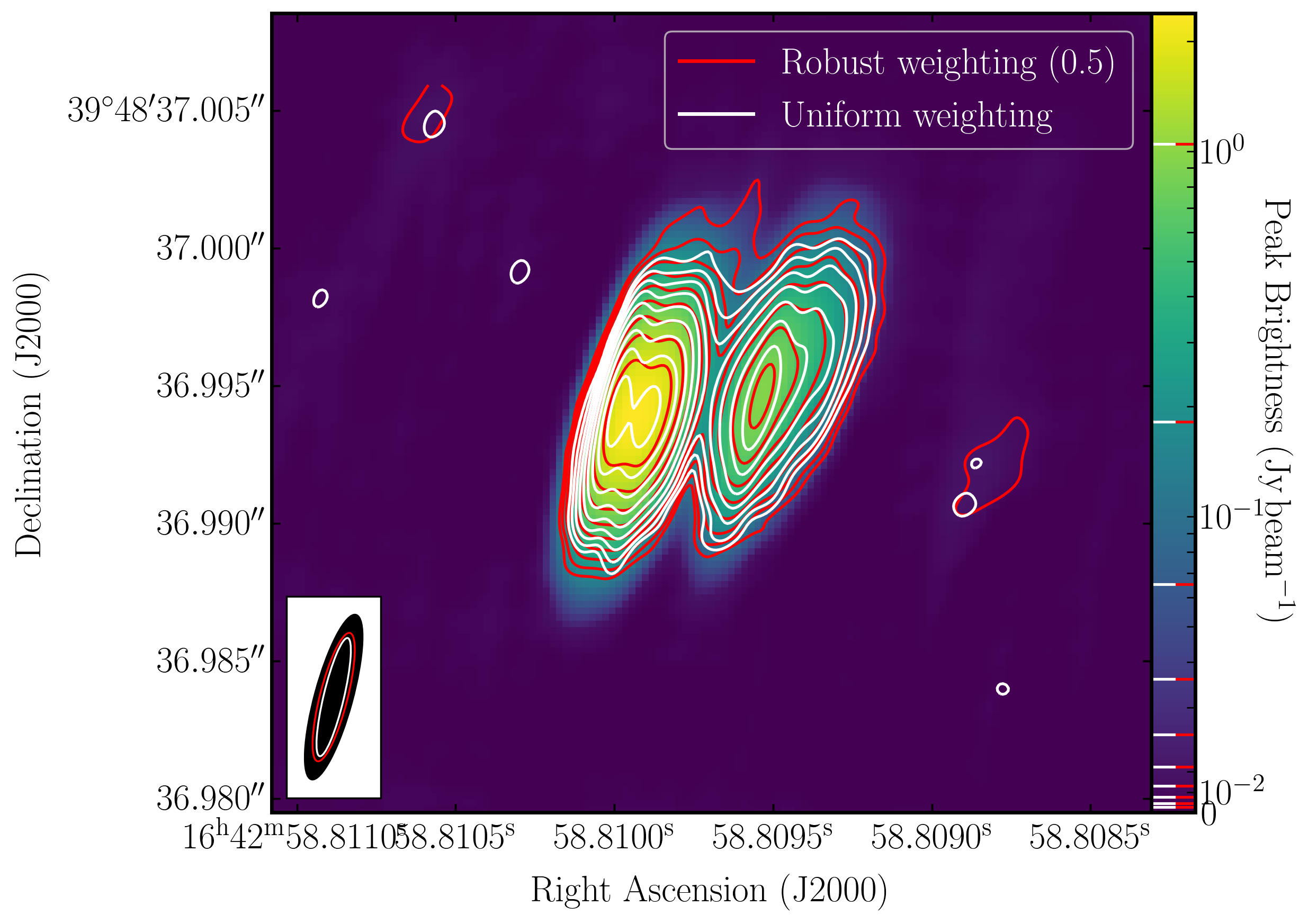
The robustly weighted image offers a balance between the uniformly and naturally weighted images, resulting in intermediate resolutions and sensitivities. In the plot below, we have overlaid the three images using Python. The background image is the naturally weighted image, while the contours represent the re-weighted images. You can clearly see the differences in resolution (bottom left ellipses) and the structure of the source.
This concludes the EVN continuum tutorial and hopefully has provided you with insight into how to reduce VLBI data. If you would like to explore further, check out the spectral line and 3C277 e-MERLIN tutorials. If you have comments, find issues, or need extra help, please use the form below, and we will email you back as soon as possible.