Part 2: Calibration & Imaging of J1849+3024

This section assumes you have completed part 1 of the EVN Continuum tutorial. As a result of that section, you should have learnt the basics of fringe-fitting, data inspection, and bandpass calibration. In the following section, we will refine our calibration and imaging techniques. By the end of this section, we should have an image of our target sources.

While in the previous section we used CASA interactively, this section will rely on scripting your own calibration script. Generating a script to calibrate your data is advantageous because you can reproduce the calibrated data in the future in case of accidental deletion or corruption. We advise that if you are unfamiliar with Python, you should sit near someone who is, or if you are working remotely, take a look at the computing courses on the DARA webpage.

Table of contents

1. Data and supporting material
2. Scripting in CASA
3. Imaging the phase calibrator
1. Imaging 101
2. Determining the image parameters
3. Inputting the parameters and executing tclean
4. CLEANing in tclean
5. Tracking calibration improvements
4. Correct residual delay & phase errors
1. Generating the model visibilities
2. Refine delay corrections
3. Refining the phases
4. Apply corrections to the phase calibrator
5. Correct amplitude errors on the phase calibrator
1. Re-image the phase calibrator
2. Obtain amplitude solutions
3. Apply amplitude solutions
4. Re-image the phase calibrator with amplitude solutions applied
5. Apply solutions to the target
6. Split target
6. Self calibration of target
1. First target image
2. Phase self-calibration solution interval
3. Derive phase self-calibration solutions
4. Apply and image target again
5. Inspect target structure
6. Amplitude self-calibration
7. Final imaging

1. Data and supporting material

For this section, you will need the scripts found in EVN_continuum_pt2_scripts_casa6.tar.gz (the download link is on the workshop homepage) and the $uv$ data set - 1848+283_J1849+3024.ms - from part 1. Organise these two files into separate folders to easily distinguish between parts 1, 2, and 3 of this tutorial, and extract the scripts. You should have the following in your folder:

• 1848+283_J1849+3024.ms - partially calibrated $uv$ data. Please note that if you encounter unusual results when using the data from part 1, you should download the $uv$ data (EVN_continuum_pt2_uv_casa6.tar.gz) using the link on the homepage.
• NME_J1849.py - complete calibration script to use as a reference or if you get stuck.
• NME_J1849_skeleton.py - calibration script we will input values into.

2. Scripting in CASA

The CASA calibration package allows you to create your own scripts that can be executed in the CASA prompt or from the command line. You will recall from part 1 that we executed some scripts (e.g., append_tsys.py and gc.py) in the command line using the -c argument. In this section, we will execute scripts from within the CASA prompt.

To start, please do the following:

• Open both files NME_1849.py and NME_1849_skeleton.py using a text editor, such as gedit. Use NME_1849_skeleton.py to input our commands, while NME_1849.py will serve as the guide. Please do not copy and paste between the two files, as you won't learn anything!
• Open a CASA interactive prompt by typing casa in the command line.

Examine the NME_1849_skeleton.py file. This file provides an example of a CASA calibration script. The script is designed so that only a subset of commands is executed at any given time (keep in mind that there are various ways to achieve this!). This approach is beneficial because it allows us to test and run small sections of the scripts to ensure correctness, rather than wasting time executing all commands simultaneously only to discover numerous mistakes along the way. Let's examine the preamble to see how this is accomplished.

Lines 13-19:

import os, sys

if (sys.platform == 'darwin'): ## this is a bit of code to deal with the viewer issue
	mac = True
	from casagui.apps import run_iclean
else:
	mac = False

As usual with Python scripts, the imported libraries like os and sys are at the top of the script. CASA is a self-contained Python environment, so you can install other libraries by using !pip3 install <library> in the CASA prompt. The if statement simply allows the code to determine whether you are using a Mac, so it can use a different method for interactive imaging later (as the historical CASA method no longer works on Macs).

Lines 39-43:

### Inputs ###########
target='J1849+3024'
phscal='1848+283'
antref='EF'                  # refant as origin of phase
######################

One of the main advantages of scripting is that we can set variables to be used throughout the entire script. While the calibration may remain similar for many data sets, these variables often differ between data sets but are common within the script, such as targets, phase calibrators, experiment names, and antennas. By setting such variables, we only need to adjust a few lines of code to adapt these scripts to other data. In this case, we are setting the target name, phase calibrator name, and reference antenna as variables, because they will be used multiple times.

Lines 40-78:

thesteps = []
step_title = {1: 'Image phase cal',
			  2: 'Obtain image information',
			  3: 'FT phase cal to generate model',
			  4: 'Refine delay calibration',
			  5: 'Refine phase calibration',
			  6: 'Apply all calibration to phasecal',
			  7: 'Re-image phasecal',
			  8: 'Phasecal selfcal in amp and phase',
			  9: 'Apply solutions to phasecal',
			  10: 'Re-image phasecal with selfcal done',
			  11: 'Apply solutions to target',
			  12: 'Split target from ms',
			  13: 'Image target w/ calibration from phase referencing',
			  14: 'Look at structure of target',
			  15: 'Phase only self-cal on target',
			  16: 'Apply + generate new model',
			  17: 'Look at structure of target w/ phase self-cal',
			  18: 'Amp+phase self-cal on target',
			  19: 'Apply and make science image'
}

try:
	print('List of steps to be executed ...', runsteps)
	thesteps = runsteps
except:
	print('global variable runsteps not set')

print(runsteps)

if (thesteps==[]):
	thesteps = range(0,len(step_title))
	print('Executing all steps: ', thesteps)

### 1) Image phase calibrator
mystep = 1

if(mystep in thesteps):
	print('Step ', mystep, step_title[mystep])

This section of code tests your newfound Python knowledge. First, try to figure out what each individual part does on your own, and then read on to see if you were correct!

This section of the code establishes how we can divide the script into smaller segments, allowing us to test and execute only individual parts. Let's explore their significance:

• Line 46 initialises the thesteps variable as an empty array. This array dictates which blocks of code are executed!
• Lines 47-66 generates a Python dictionary named step_title that provides information on what each sub-step of the tasks does. The keys in the dictionary will correspond to the step numbers performed.
• Lines 68-72: this try/except statement defines which blocks of code will be executed. If you look closely, the user needs to define the runsteps parameter before running the script; otherwise, the script will cause an error and print the string in the except statement.
• Lines 76-78: If runsteps=[], then thesteps=[] also evaluates to the same. This snippet of code thus assigns the thesteps parameter the value [0,1,2,3,...,19], ensuring that all tasks are executed.
• Lines 80-84: this piece of code serves as the preamble for each block of tasks executed. The setting of the integer variable mystep determines the step number. The if statement checks whether this mystep integer is included in the steps specified by the user, which is determined by the runsteps parameter. If this condition is met (i.e. mystep in thesteps = True), then the indented if statement executes, printing the title of this step along with the tasks within the indented block of code. You will notice that this preamble defines the breakpoints of each section of code.

Keeping this in mind, the method for using this code within CASA becomes evident. The user must define the parameter runsteps=[<task number>], and then we can execute the script with the execfile() function. For instance, to run steps 1 and 3, we would enter the following into the CASA interactive prompt:

runsteps = [1,3]
execfile('NME_J1849_skeleton.py')

Let's begin the tutorial. The first few steps will consist of only one CASA task at a time to minimise mistakes when entering the parameters. By the end, you should be able to conduct multiple tasks simultaneously, as you should have a good understanding of the parameters to be inputted by then.

3. Imaging the phase calibrator

← back to top

As previously stated in Part 1, we assumed the phase calibrator is point-like (i.e., with the same amplitude on all baselines and zero phase). However, in VLBI arrays, many calibrators are slightly resolved. Imaging the phase reference source is always a useful step.

The image of the phase calibrator requires us to use the task tclean in step 1 of the NME_1849_skeleton.py code. If you are working on a Mac, we will need to use run_iclean, which is simply a wrapper around tclean to enable the interactive imaging capabilities.

By now in your course, you should have received an introduction to imaging; however, the next sub-section will recap it.

3A. Imaging 101

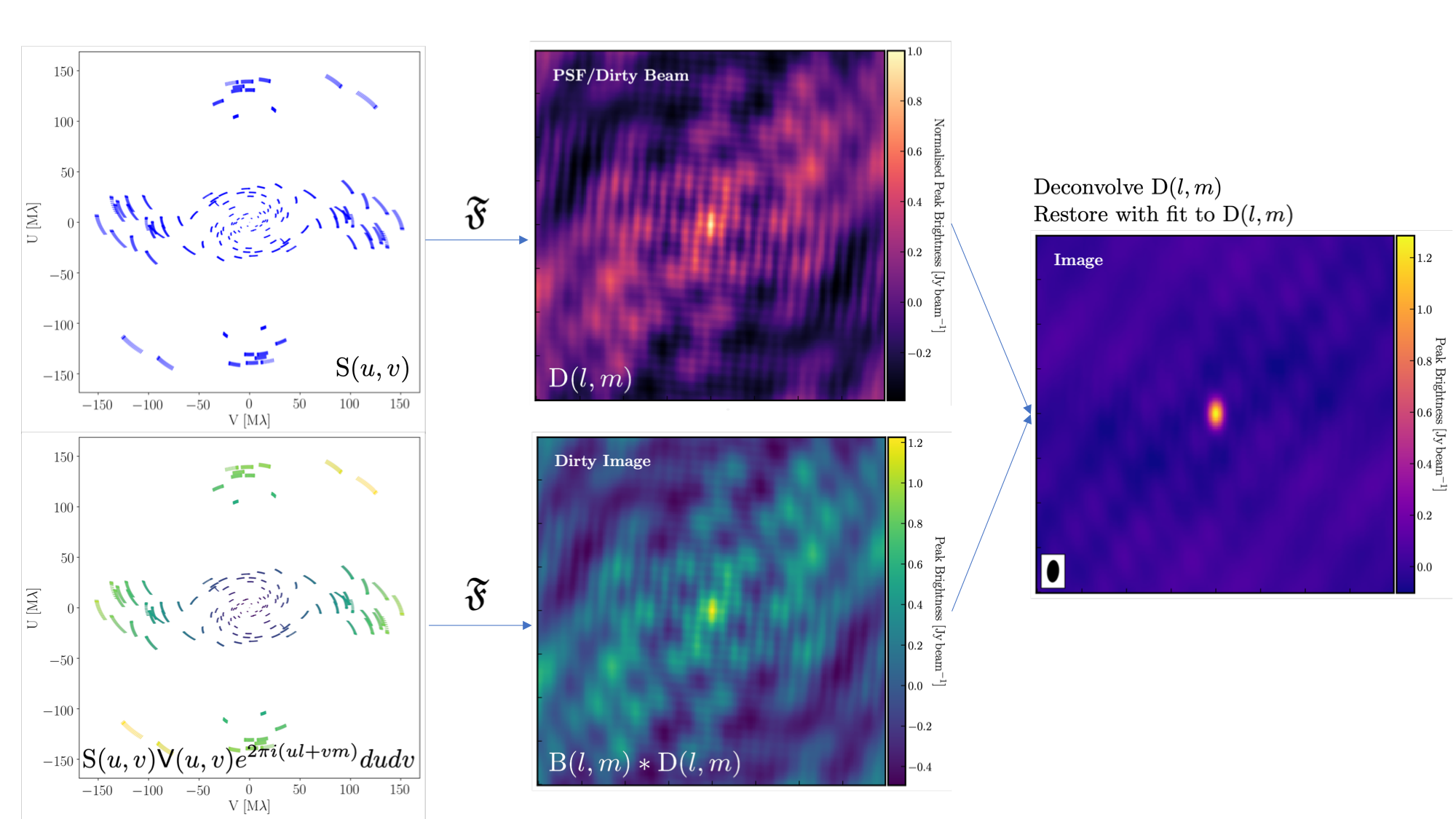
The figure above summarises the imaging process, using our phase calibrator as an example, and we will discuss this in the following section. If you recall from the lectures, we can represent the visibilities measured by an interferometer, $\mathsf{V} ( u , v )$, with the following equation, $$\mathsf{V} ( u , v ) \approx \iint _ { l m } \mathsf { B } ( l , m ) e ^ { - 2 \pi i ( u l + v m ) } \mathrm{d}l \mathrm{d}m,$$ where $\mathsf { B } ( l , m )$ represents the sky brightness distribution, $ l$ and $ m$ are the directional cosines on the sky, and $u$ and $v$ denote the projected baseline vectors (and their conjugates). From the lectures, you will recall that a key factor in interferometric observations is that we have an unfilled $uv$ plane; that is, we are not sensitive to all spatial frequencies. This makes imaging a fundamentally more difficult problem because we must deal with arrays that have 'holes' in them (also referred to as sparse arrays). Consequently, directly performing a Fourier transform on the visibilities becomes nearly impossible.

To get around this, we define a sampling function, $\mathsf{S}(u,v)$, which equals 1 when there is a measurement on the $uv$ plane and 0 otherwise. The sampling function is straightforward to determine because we know exactly where our antennas are positioned at all times, and consequently, we know the locations they will occupy on the $uv$ plane. A good way to visualise the $uv$ plane is to imagine the apparent movement of the antennas throughout the observations, as if you were observing the Earth from the location of the source.

If we multiply both sides of the imaging equation by the inverse Fourier Transform of the sampling function, we can apply the Fourier Transform ($\mathfrak{F}$) to the imaging equation, resulting in, $$\mathsf{ B } ( l , m ) * \mathsf{ D } ( l , m ) \approx \iint _ { uv } \mathsf{S} ( u , v ) \mathsf{V}( u , v ) e ^ { 2 \pi i ( u l + v m ) } \mathrm{d}u\mathrm{d}v, \\\mathrm{where~~}\mathsf{ D } ( l , m ) = \iint _ { u v } \mathsf{S} ( u , v ) e ^ { 2 \pi i ( u l + v m ) } \mathrm{d}u \mathrm{d}v,$$ where $\ast$ is the convolution operator. You can see that we can now recover the intrinsic source brightness distribution $\mathsf{B}(l,m)$ if we can deconvolve the $\mathsf{D}(l,m)$ term from it. This $\mathsf{D}(l,m)$ term is known as the dirty beam or point spread function (PSF). Fortunately, this can be easily derived because we know exactly what $\mathsf{S}(u,v)$ is.

Sounds simple, eh? Not so! The next step, namely the deconvolution of the PSF from the dirty image, is a bit more complicated than it sounds. The deconvolution process is referred to as an 'ill-posed' problem in mathematics. This means that, without some assumptions, solutions to deconvolution are often not unique, i.e., there are many variants of the sky brightness, $\mathsf{B}(l,m)$, that would satisfy the equation. Additionally, the algorithms used to perform deconvolution are non-linear and may diverge from 'good' solutions.

To aid the deconvolution process, we can apply a range of assumptions to guide it toward the most likely sky brightness distribution. These assumptions are often based on physical principles, such as the requirement that $\mathsf{B}(l,m)$ is always positive; however, the specifics can vary with each different deconvolution algorithm.

The most commonly used string of algorithms is the CLEAN variants, which we shall discuss here. The standard CLEAN algorithm (either Högbom or Clark) assumes that the sky is sparse, meaning that radio sources are far from each other, and that the sky brightness distribution can be represented by point sources (i.e., delta functions). The CLEAN algorithm goes through many cycles in which it identifies the brightest pixels, removes 10% (the default value) of the flux density at each of these pixels, and records the value and position in a model image. CLEAN then calculates the contribution of these removed pixels by convolving the removed flux it with the PSF, and then subtracts it from the dirty image. This is known as a 'minor cycle.'

After a certain number of minor cycles, the model is Fourier transformed and subtracted from the visibility data, which is then re-Fourier transformed to create a new dirty image that has less bright emission and fewer contributions from the dirty beam. This process is known as a 'major cycle'. These cycles continue until the final dirty image (or 'residual image') is indistinguishable from noise. The following GIF demonstrates the CLEAN process on the 1848+283 phase calibrator we are about to image. You can see how the model is built up and how the contribution from the PSF decreases with each major cycle and each CLEAN iteration (which removes 10% from the brightest pixel).

Once deconvolution is complete and the residual image appears close to noise, the model is convolved with the synthesised beam and added back into the data (without the undesirable PSF sidelobes). The synthesised or restoring beam is an idealised Gaussian fit to the PSF and can be considered the effective resolution of the interferometer array. The final image is shown in the rightmost panel of the figure at the beginning of this section. The synthesised beam size is represented by the elliptical overlay in the bottom left corner of the figure.

3B. Determining the imaging parameters

← back to top

Let's proceed with creating our first image using the CASA task tclean. In the CASA prompt, type default(tclean) followed by inp. If you are using a Mac, note that run_iclean task we will use takes the same arguments as tclean, with identical meanings. There are quite a few inputs which can seem daunting; however, this task is very versatile and performs imaging for many different use cases (e.g., spectral line, wide-field, etc.). If you are unsure what is best for your data, consult the CASA documentation.

There are, however, some things we always need to decide and set when imaging, which are:

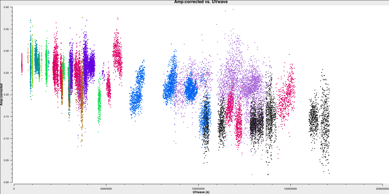
1. imagename - this is self-explanatory; you need to set an image name that describes the imaging step and the object being imaged.

2. field - this is the name of the field you want to observe, and it is, once again, self-explanatory.

3. cell - this is the angular size of each pixel in our output image. To estimate this, we need to determine the resolution of our interferometer. We can do this by examining the $uv$ distance (i.e., the radial distance of measurements in the $uv$ plane). In CASA, type the following commands:

   default(plotms)
   vis='1848+283_J1849+3024.ms'
   xaxis='uvwave'
   yaxis='amp'
   field='1848+283'
   antenna="*&*"
   spw='7'
   correlation='RR'
   plotms()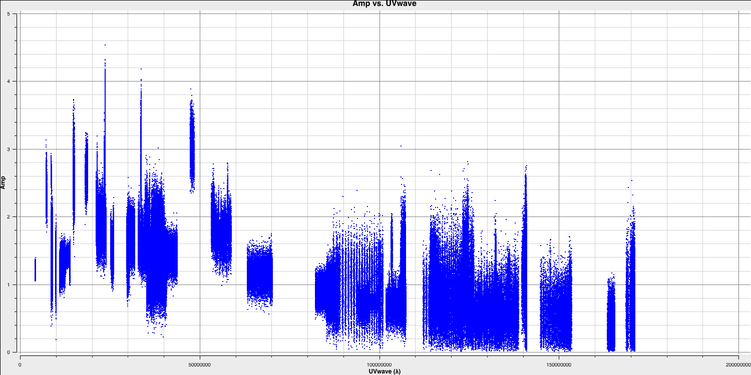

   

   Only the highest frequency spectral window is chosen, as this corresponds to the best resolution (remember the resolution is $\propto \lambda$), and only one correlation is selected. These choices are made to improve the plotting timescale. Note that we have used some other parameters in plotms to plot gridlines.

   To obtain a good value for cell size, you should read the highest $uv$ distance value, which is approximately $1.7\times10^{8}\,\lambda$. With this obtained, we can convert these values into a resolution (remember that the resolution of an interferometer is $\sim{\lambda}/B$ and the $\lambda$s will cancel out!).

   There is one other factor that we have overlooked, and that is Nyquist sampling ($N_\mathrm{s}$). During imaging, we need to fit a 2D Gaussian to the PSF to estimate the instrument's resolution if the aperture is fully filled. This is referred to as the synthesised/restoring beam. The minimum number of pixels spanning the Gaussian to achieve a fit must be at least 3 pixels, but often (especially in VLBI, where the PSFs are highly non-Gaussian) more pixels are used.

   Based on the aforementioned points, an estimate for an appropriate cell size can be expressed using the following equation, $$\mathrm{cell} \approx \frac{180}{\pi N_\mathrm{s}} \times \frac{1}{D_\mathrm{max}\,\mathrm{[\lambda]}}~\mathrm{[deg]}.$$

   Assuming a $D_\mathrm{max} = 1.7\times10^{8}\,\lambda$ and $N_\mathrm{s}$ of 5 pixels, this case suggests that you will obtain a cell size of approximately $0.24\,\mathrm{mas}$, i.e., cell=['0.24mas'].

4. imsize - this describes the number of pixels on each side of your image. Often, this involves a compromise between computing speed and deconvolution performance. You want an image that is not too large but is sufficiently sized to allow for the removal of the PSF sidelobes (see the imaging figure above!). If your source is extended, the image size may also need to be larger to accommodate this. Additionally, we want to select an image size that is optimal for the underlying algorithms in tclean. According to CASA, a suitable number to choose should be even and divisible by only 2, 3, 5, and 7. An easy rule of thumb is to use an image size of $2^{n}\times 10$, where $n$ is an integer, such as 80, 160, 320, 640, 1280, 2560, or 5120. In this case, we are adopting an image size of 640, i.e., imsize=[640,640]

5. deconvolver - the choice of deconvolution algorithm is highly dependent on your source and your interferometer. To establish the correct choice for your data, consult the CASA documentation. A good rule of thumb for what to pick is the following:

   • Do you expect that your sources are extended, i.e., $\gg$ the resolution? Consider multiscale. This deconvolution algorithm assumes the sky consists of many Gaussians, which is better for modelling fluffy emission compared to using delta functions.
   • Does your observation have a large fractional bandwidth? A good rule of thumb is total bandwidth divided by central frequency, i.e., $\mathrm{BW}/\nu_c > 10\%$. Consider mtmfs (this models the change in flux/morphology of the source across the bandwidth; failures to model this can cause un-deconvolvable errors in the image). If the source is also extended, implement multiscale deconvolution by setting the scales parameter.
   • Do you expect the source to have structure in polarisation? Consider clarkstokes, which cleans the separate polarisations individually.
   • If not, then we would expect to have a small bandwidth and compact structure; therefore, the clark algorithm should be sufficient.

   In our case, the phase calibrator (by definition!) should be compact. We have a small fractional bandwidth ($\mathrm{BW}/\nu_c \sim 0.128\,\mathrm{GHz}/5\,\mathrm{GHz} \sim \mathbf{2.6\%}$), and we don't care about polarisation here. This means that setting deconvolver='clark' should be fine.

6. niter - following the setup of the deconvolver, this parameter determines the number of iterations that the deconvolution algorithm will use. If you recall from earlier, for each iteration, a percentage of the flux from the brightest pixel is removed from the dirty image; therefore, the larger the niter, the more flux is removed. Fortunately, we will perform this interactively and inspect the residuals after each major cycle, allowing us to adjust niter on the fly. As such, we won't go too deep, so we set niter=1000 and use interactive=True to enable interactive adjustments.

7. weighting - The weighting parameter determines how the various baselines are represented in the imaging routine. Uniform weighting gives each baseline in the $uv$ plane equal weight, typically resulting in images with the highest resolution. In contrast, natural weighting maximises sensitivity and enhances the contributions from data points and baselines that are closer in the $uv$ plane. For this imaging, we will use the default of weighting='natural'. We will examine the effects of changing the weighting in the 3C277.1 data reduction workshop and in Part 3 of this workshop.

3C. Inputting the parameters and executing tclean

← back to top

Now that we have determined the parameters to set and the values to use, let's input these into our NME_J1849_skeleton.py script. Note that the code blocks are divided based on your operating system.

• Go to step 1 in NME_J1849_skeleton.py and you should find the following:

### 1) Image phase calibrator
mystep = 1

if(mystep in thesteps):
	print('Step ', mystep, step_title[mystep])

	# Image the phase calibrator with tclean

	os.system('rm -r '+phscal+'_p0.*')

	if mac==False:
		tclean(vis=phscal+'_'+target+'.ms',
			imagename='phasecal1p0',
			stokes='pseudoI',
			psfcutoff=0.5,
			specmode='mfs',
			threshold=0,
			field='xxx',
			imsize=['xxx','xxx'],
			cell=['xxx'],
			gridder='xxx',
			deconvolver='xxx',
			niter='xxx',
			interactive=True)

	else:
		run_iclean(vis=phscal+'_'+target+'.ms',
				   imagename='phasecal1p0',
				   stokes='pseudoI',
				   specmode='mfs',
				   threshold=0,
				   field='xxx',
				   imsize=['xxx','xxx'],
				   cell=['xxx'],
				   gridder='xxx',
				   deconvolver='xxx',
				   niter='xxx')

• Replace the 'xxx' in the relevant task (tclean if on Linux or run_iclean on macOS systems) with the imaging parameters that we have just derived. Remember to check tclean (using inp tclean and help tclean) to ensure that the included variables are in the correct format, e.g., imsize=[<integer>,<integer>] and not strings!
• Some final comments on additional parameters. The use of stokes='pseudoI' ensures that the telescope with a single observed polarisation (e.g., Svetloe / SV) is included when imaging, improving sensitivity. To generate true Stokes $I$ images, we need to combine both RR and LL ($I = (RR + LL)/2$). The pseudo Stokes $I$ assumes equal power in the unobserved polarisation. While this is acceptable for non-polarimetric imaging like this case, we should avoid using pseudoI for polarisation studies. Additionally, the use of psfcutoff=0.5 ensures that the highly irregular PSF is fitted properly. Note that this parameter is not used in the run_iclean task as it is not supported.
• Run this block of code in the CASA prompt using the syntax we introduced earlier, i.e.,

  ## In the CASA prompt
  	runsteps = [1]
  	execfile('NME_J1849_skeleton.py')

• If you encounter errors, compare your input to step 1 in NME_J1849.py to identify where you went wrong. It's often just a matter of a missing comma or incorrect indentation.

3D. CLEANing in tclean

← back to top

Now that you have executed (Linux) tclean / (macOS) run_iclean, you should notice increased activity in the logger. The algorithm will grid the visibilities with the appropriate weights and produce the PSF, which is prepared for deconvolution and inversion of the visibilities to create our dirty image. We can guide the deconvolution process to ensure it does not diverge (as explained in part A of this section).

Guidance comes from the use of masks. These masks instruct CLEAN on which pixels to search for the flux to be removed and the PSF to be deconvolved. The masks should be applied in regions where you believe there is real flux. These typically resemble the shape of the PSF in the case of point sources (see part A of this section for the PSF shape). Since we set (Linux) interactive=True / (macOS) are using run_iclean, CASA returns a GUI similar to those shown below, where we can set masks and guide the deconvolution process.

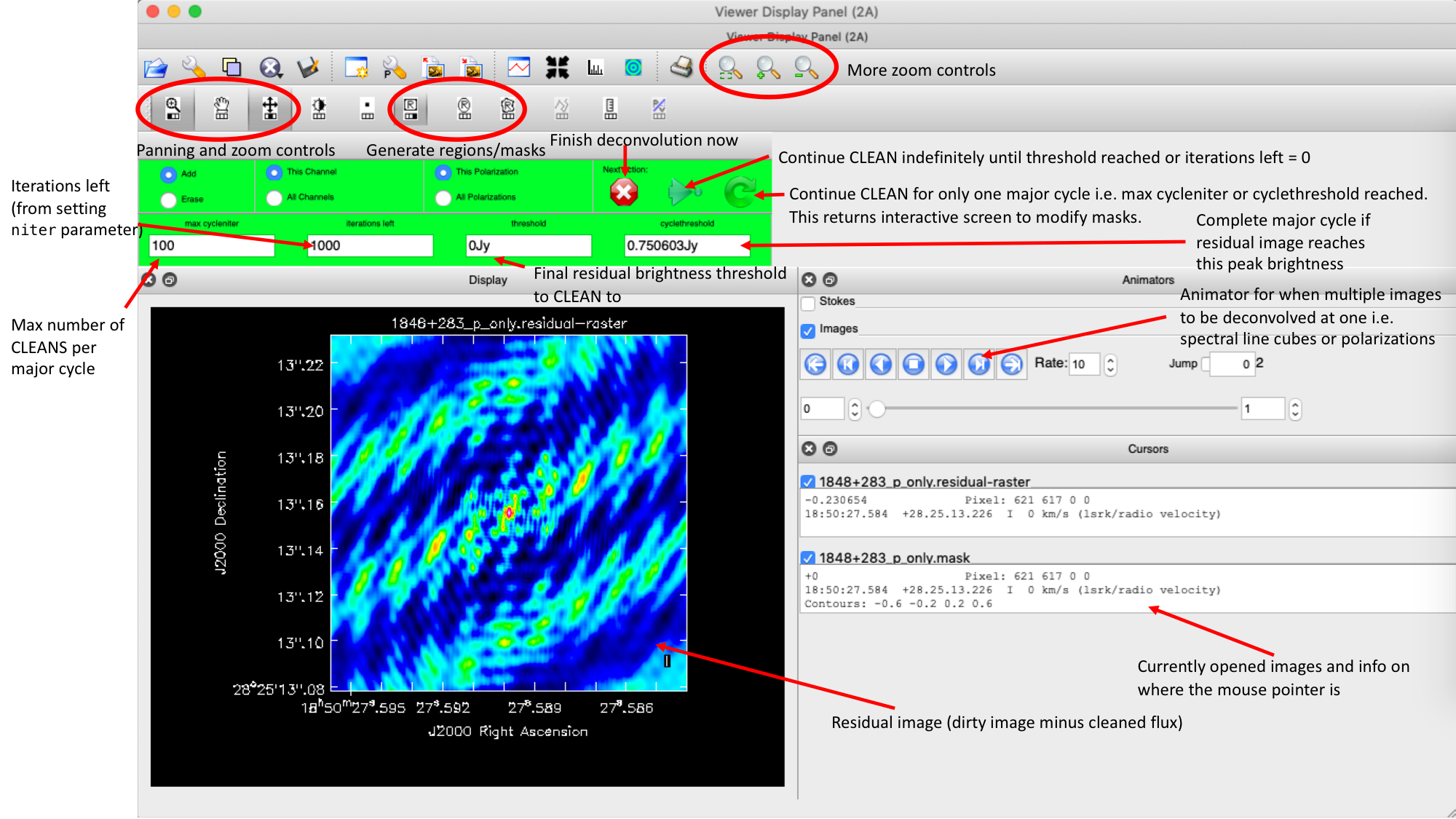
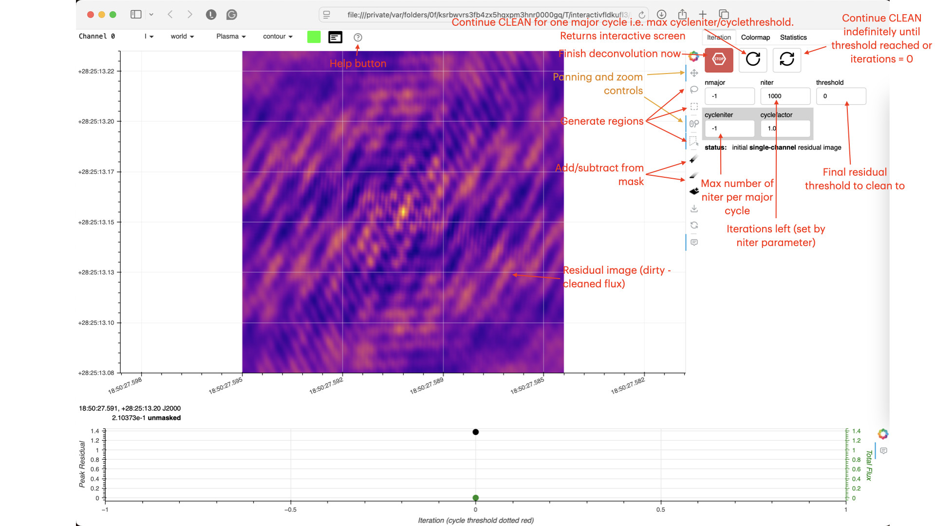
The GUI will display the dirty image. At the centre of the image, a bright source with the characteristic PSF shape surrounds it. This is where we want to start setting our mask.

• To set the mask, we want to use the region buttons (e.g. (Linux) / (macOS) ). (Linux) The filled rectangle among the three rectangles on these buttons corresponds to the mouse buttons. These can be adjusted and reassigned to different mouse buttons by clicking on them.
• (Linux) The gif below demonstrates how to set the mask and run the next major cycle. IMPORTANT: To set the mask, we need to (Linux) double-click with the appropriate button (in this case, the right mouse button) or (macOS) press Shift+A, and the box should change to a solid line. Set a mask around the obviously brightest regions and clean interactively; mask new regions or increase the mask size as needed.
  
• Once the (Linux) green arrow button or (macOS) single circular arrow has been pressed, the next major cycle will run, causing the GUI to freeze. This process will remove some flux, deconvolve the PSF, and begin generating the model as explained in part A. After these contributions have been removed from the visibilities, the task will generate another residual image with less bright flux and will reopen the GUI.
• Continue with the CLEANing process and modify the mask as appropriate. Note that you can delete parts of the mask by either (Linux) clicking on the erase button, overlaying the green box on the area to remove, and double-clicking to delete that portion, or (macOS) by drawing a region and pressing the subtract button.
• Throughout the CLEAN process, you should observe the PSF imprint being removed and the residual transforming into noise (or noise plus calibration errors). Below, we present the GIF again from part A to illustrate what you should see at the end of each major cycle in your GUI.
  
• After approximately three major cycles, you should observe some low flux density structures appear, indicating that our phase calibrator is not a true point source, so the assumption from Part 1 is slightly incorrect. We will soon use the model generated with CLEAN to correct for this!
• Continue until approximately major cycle 6, where the source becomes indistinguishable from noise, and click the red stop button to halt cleaning.

With CLEAN stopped and completed, the algorithm will take the model image (the delta functions), convolve it with the fitted PSF, or the synthesised beam, and add this to the residual image to generate the final image. Let's examine what CLEAN has produced:

• Type !ls into the CASA prompt.
• You should see some new files which are CASA images. These are:
  • phasecal1p0.image - the model convolved with the synthesised beam added into the residual image.
  • phasecal1p0.residual - the noise image after CLEAN deconvolution (seen in the interactive prompt during CLEANing).
  • phasecal1p0.model - the underlying estimated sky brightness model by CLEAN.
  • phasecal1p0.psf - the FT of the sampling function that is deconvolved.
  • phasecal1p0.pb - the primary beam response across the image (Note this is not correct for heterogeneous arrays yet).
  • phasecal1p0.sumwt - the sum of weights (not needed).
• (Linux only) Enter imview at the CASA prompt or (macOS & Linux) open CARTA and examine these images. Attempt to determine the origin of these images by comparing them to the imaging description presented in part A.
• Inspect the phasecal1p0.image. The source appears quite point-like, but the background noise shows a distinctly non-Gaussian pattern, with visible stripes and negatives arranged in a non-random manner. This serves as a clear indication of calibration errors. Such issues are anticipated, as we have neither corrected for any amplitude errors nor considered the slight non-point-like nature of our calibrator.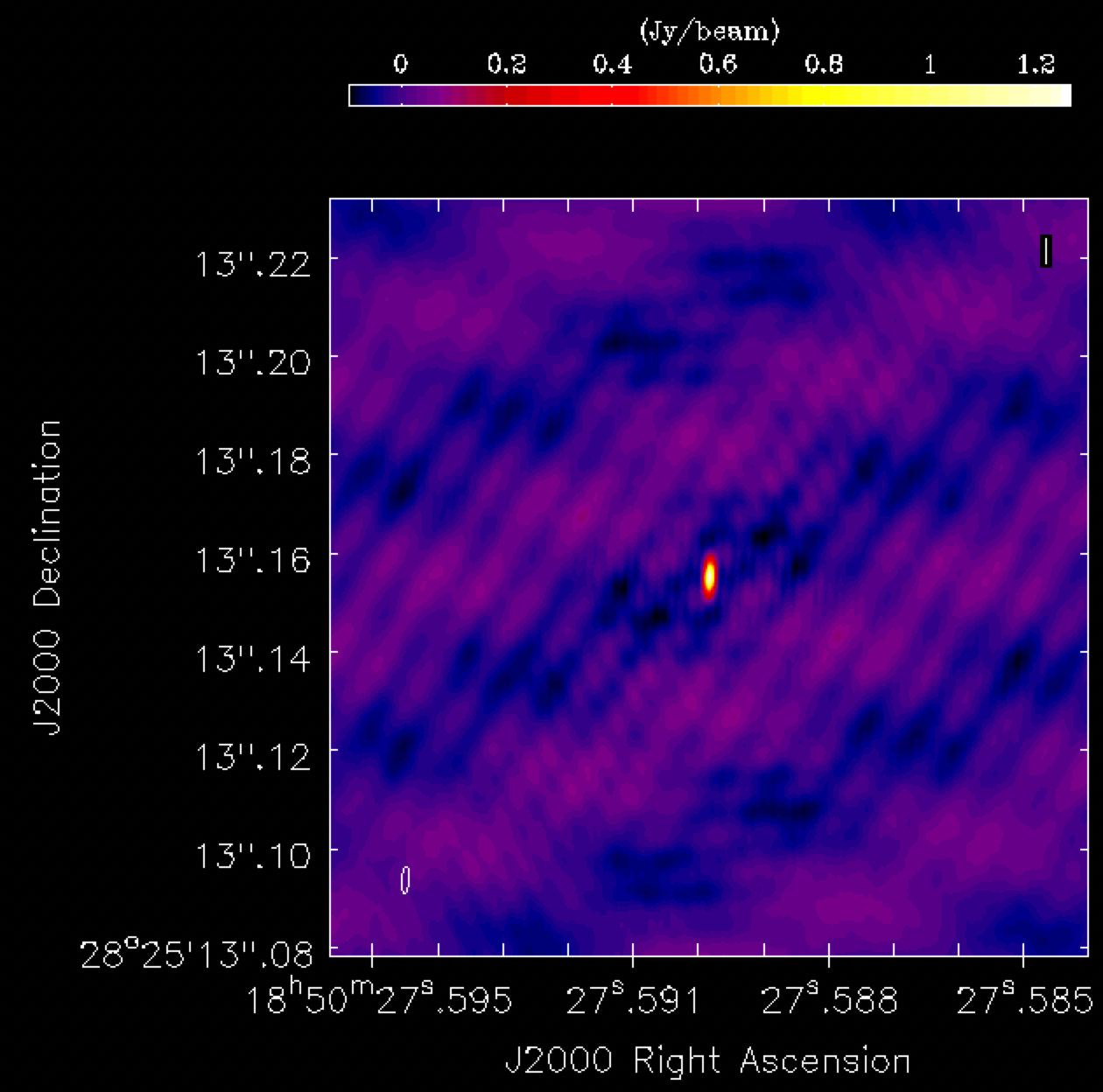
  
• Select and open the phasecal1p0.model, as this will show the non-point like nature of the object.

3E. Tracking calibration improvements

← back to top

A key step to improving calibration is tracking enhancements in image fidelity. This can be achieved by measuring the peak brightness ($S_p$), the r.m.s. noise ($\sigma$), and the signal-to-noise ratio ($\mathrm{S/N} = S_p/\sigma$).

Calibration errors typically cause flux to disperse into the noise, thereby increasing it and reducing the S/N. We can gauge whether our calibration- scheduled for the next steps- is effective by tracking the improvement in S/N. An increasing S/N indicates that we are recovering the mis-calibrated flux currently scattered in the noise. The peak and r.m.s. values are useful for assessing whether the amplitude calibration is functioning properly. Poor amplitude calibration can often alter the flux scaling, causing both the rms and peak to change in the same direction (which would be incorrect).

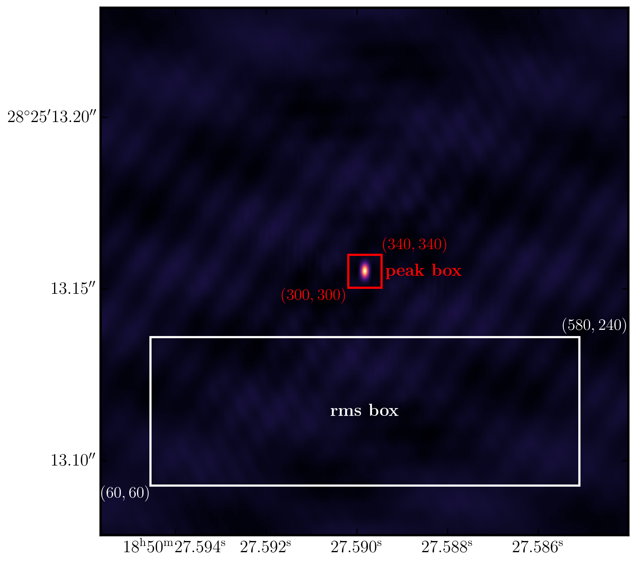
To obtain these values, we need to use the task imstat, which derives statistics from the image. To find the peak and r.m.s., we must define two boxes. The first should be located away from the source in an 'empty' area to measure the r.m.s., while the second should be positioned over the source to extract the peak pixel value.

• Look at step 2 in the script.

### 2) Get image information
mystep = 2

if(mystep in thesteps):
	print('Step ', mystep, step_title[mystep])

	# Measure the signal-to-noise
	rms=imstat(imagename='phasecal1p0.image',
			   box='xxx,xxx,xxx,xxx')['rms'][0]
	peak=imstat(imagename='phasecal1p0.image',
			   box='xxx,xxx,xxx,xxx')['max'][0]

	print('Peak %6.3f Jy/beam, rms %6.3f Jy/beam, S/N %6.0f' % (peak, rms, peak/rms))

• You can see that we need to define the two boxes by their bottom left corner (blc) and top right corner (trc) coordinates. The box parameter follows the syntax box='blcx,blcy,trcx,trcy'. Use imview or CARTA to find these boxes.
• If you are happy with your boxes then run step 2.

The plot below illustrates an example of suitable boxes for an image size of $640\times640$ pixels with a cell size of 0.24 milliarcseconds. These boxes produced a peak brightness of $S_\mathrm{p} = 1.269\,\mathrm{Jy\,beam^{-1}}$ and an rms noise of $\sigma = 0.033\,\mathrm{Jy\,beam^{-1}}$, resulting in a signal-to-noise ratio of $\mathrm{S/N} \approx 38$. You should aim for values close to this. If your results diverge, you may not have cleaned deeply enough.

4. Correct residual delay & phase errors

← back to top

Fringe-fitting should have fixed our delays and phases to the first order, and often this is sufficient for phase referencing. However, as we saw at the end of part 1, there are some baselines (mainly to SH/Sheshan) whose delay solutions are unstable. Typically, this indicates that the instrumental delay changes over the course of the observation, which may be induced by receiver or correlator problems. If the phase calibrator is not particularly bright (as is often the case), we cannot correct for this since we cannot obtain a delay solution for each spw separately. However, in this instance, the phase calibrator is bright enough, allowing us to do this.

Secondly, in VLBI observations, the phase calibrator is often not a point source; therefore, we need to derive phase corrections that represent only the atmospheric phase shifts and not any source structure (which causes non-zero phases). This means that the solutions transferred to the target reflect only the atmosphere. We have observed that this is the case for our phase calibrator, which is not a true point source; thus, we should derive corrections that take this into account. To do this, we need to use a model rather than our initial point source assumption used during fringe-fitting.

4A. Generating the model visibilities

← back to top

To generate our calibration model, we use the task ft. This task takes the CLEAN model and applies a Fourier transform to produce the $\texttt{MODEL}$ data column in the measurement set. CASA uses this information to calculate the corrections by comparing the actual visibilities with the model visibilities, rather than relying on a model of a point source.

• Review step 3 to see the task ft:

  ### 3) Generate model column for self-cal
  mystep = 3
  
  if(mystep in thesteps):
  	print('Step ', mystep, step_title[mystep])
  
  	# Fourier transform model into the visibilities
  	ft(vis=phscal+'_'+target+'.ms',
  	   field='xxx',
  	   model='xxx',
  	   usescratch=True)

• Replace the field with the phase calibrator name and the model with the model image. The usescratch option is set to True to generate a physical $\texttt{MODEL}$ column, which speeds up the processing time but consumes disk space.
• With all these set, execute step 3.

Let's examine the visibilities and the model visibilities that will be used to derive solutions.

• In the interactive CASA prompt (not the script), use plotms to plot amplitude versus $uv$ distance (in wavelength) for all baselines to Effelsberg. Use only one correlation and/or one spw if loading the plot takes a long time.
• Change the column option in the plotms GUI to the model column and the data_vector$-$model columns (go to the axes tab and use the column drop-down menu) to observe the differences between the real and model visibilities.
• Repeat for the phases.

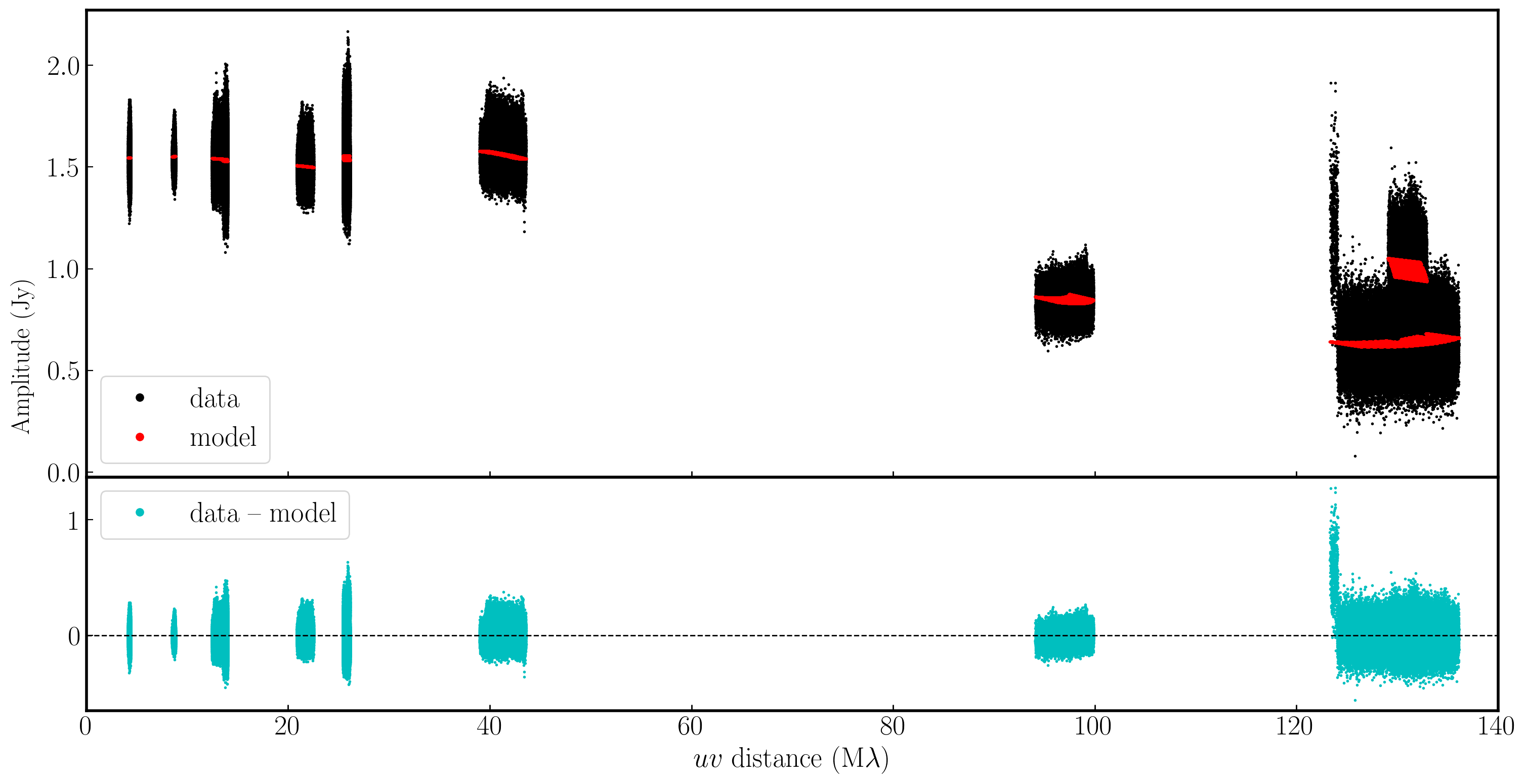
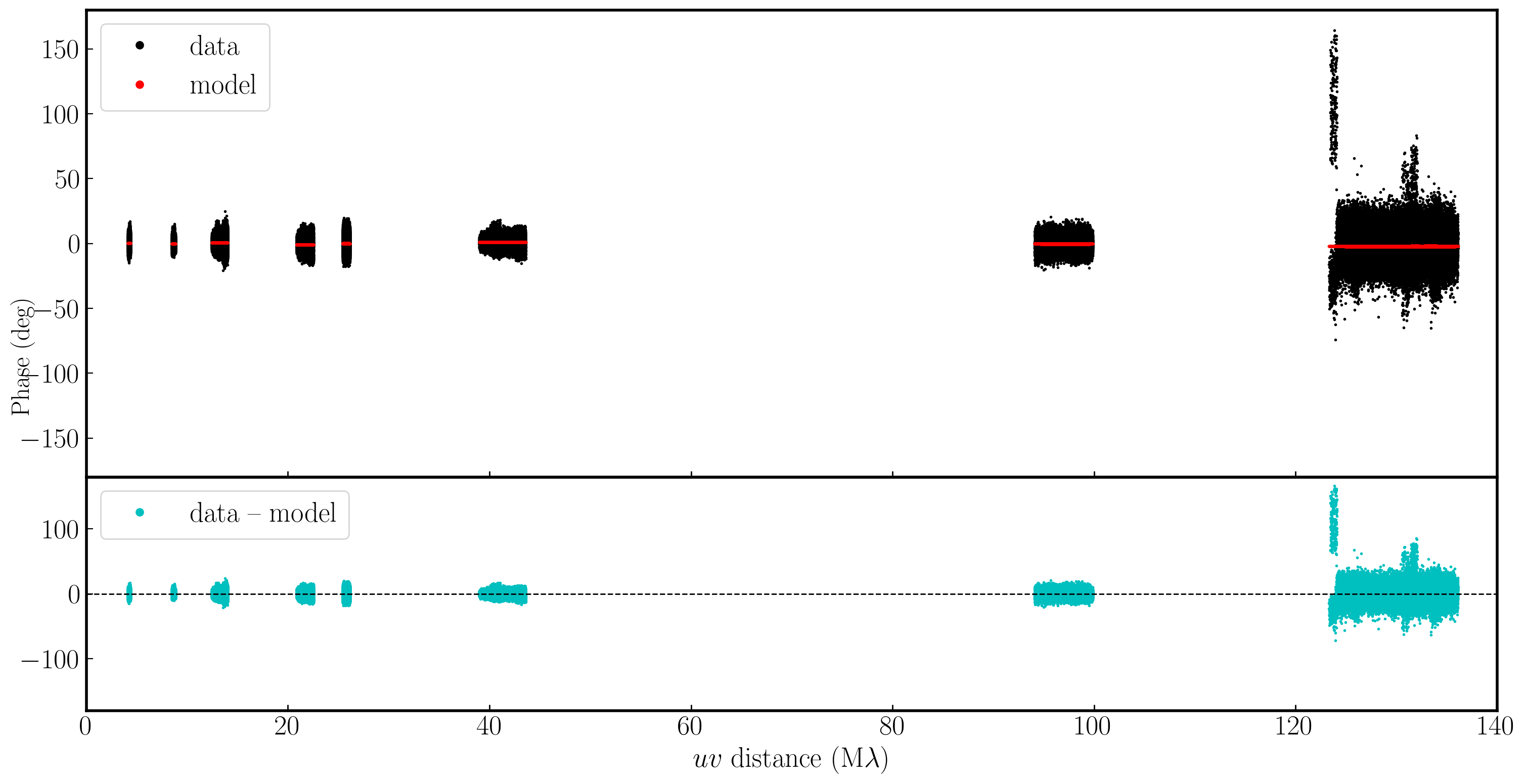
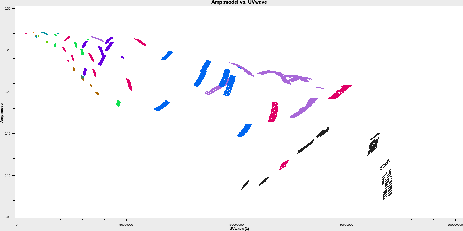
In the plot below, we have used Python to overlay the real and modeled visibilities for both amplitude and phase against uvwave (RR correlation only and all baselines to EF). The bottom panel shows the scalar subtraction of the data-model visibilities.

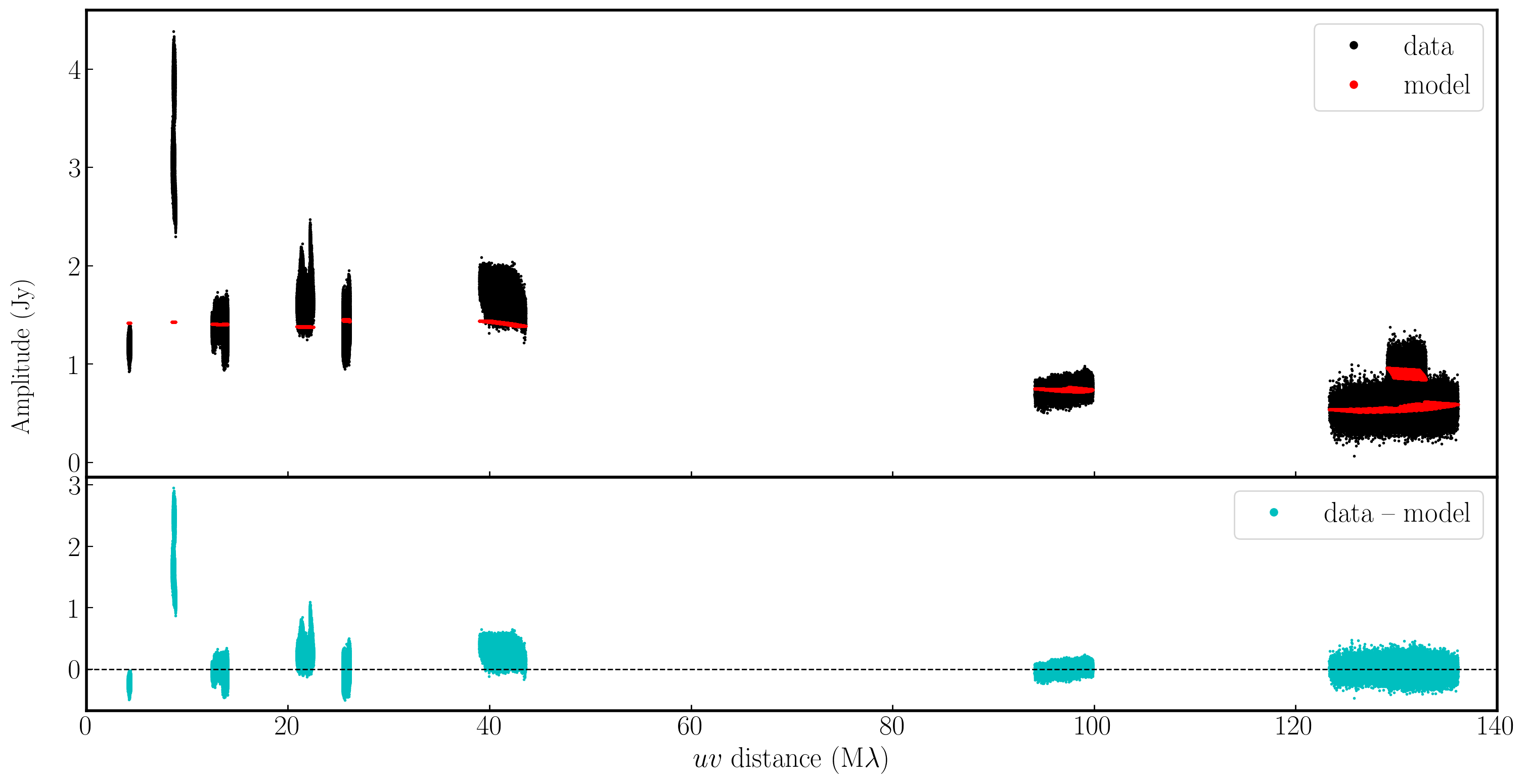
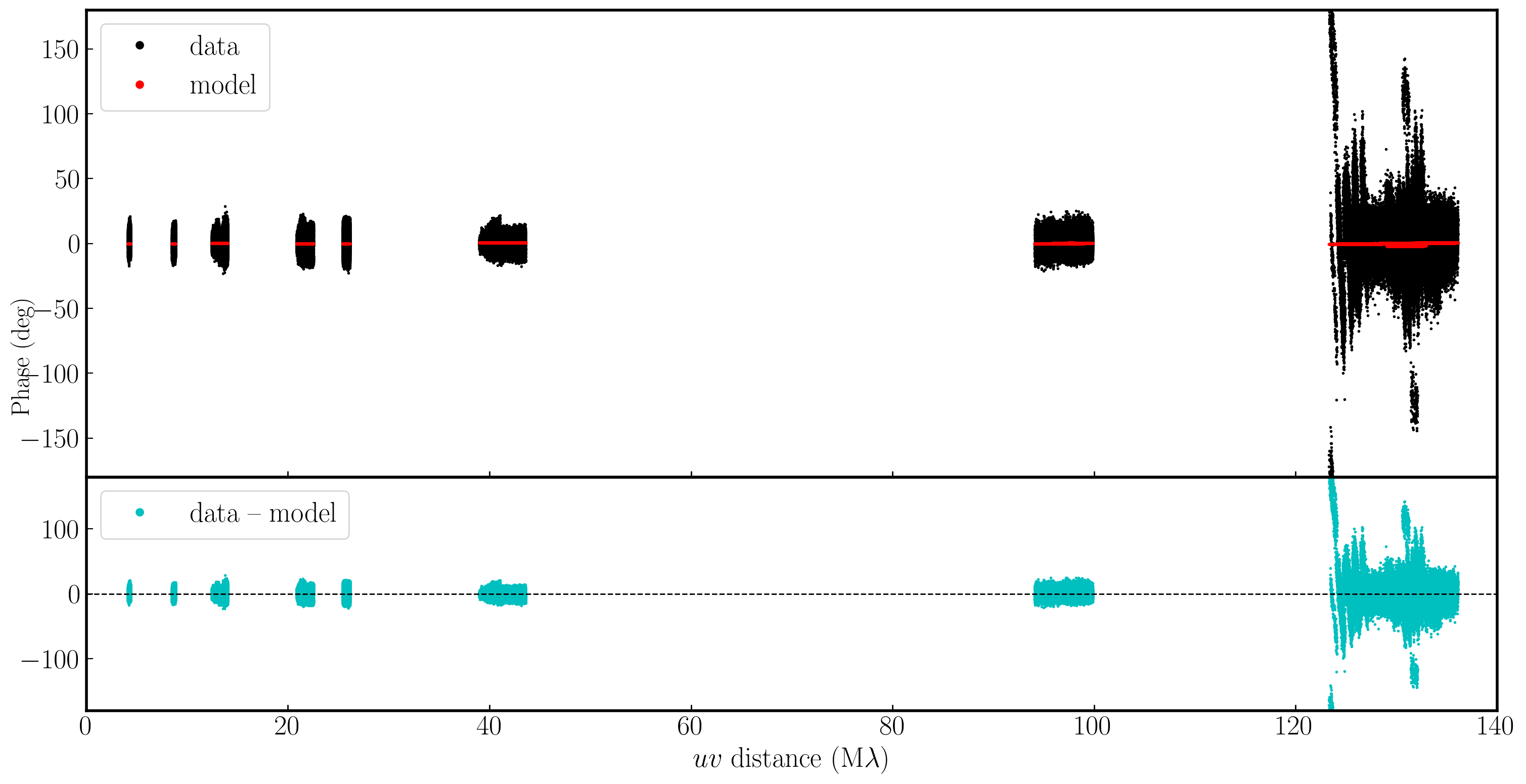
As you can see, there are large discrepancies in the amplitude versus uvwave plots. This is expected, as the initial fringe fitting in part 1 only corrects for the phases and not the amplitudes. Therefore, the phases are generally accurate compared to the model, apart from the baseline to Sheshan (approximately 120 Mλ), which has some residual delay errors that cause the phases to deviate, as we discussed earlier, and which we shall correct now!

4B. Refining the delays

← back to top

• Refer to step 4 in your skeleton file. You should see that we will use gaincal to derive our delay corrections. This multipurpose task can be employed in a myriad of ways to calibrate your data.

### 4) Refine delay calibration 
mystep = 4

if(mystep in thesteps):
	print('Step ', mystep, step_title[mystep])

	# Gain calibration of phases only
	os.system('rm -r '+phscal+'_'+target+'.K')
	gaincal(vis=phscal+'_'+target+'.ms',
			field='xxx',
			caltable=phscal+'_'+target+'.K',
			corrdepflags=True,
			solint='xxx',
			refant='xxx',
			minblperant='xxx',
			gaintype='xxx',
			parang='xxx')

	plotms(vis=phscal+'_'+target+'.K',
		   gridrows=2,
		   gridcols=3,
		   yaxis='xxx',
		   xaxis='xxx',
		   iteraxis='xxx',
		   coloraxis='xxx')

We need to set some parameters here, and the most important one is the solution interval. In this case, our phase calibrator is bright enough to obtain a solution interval for each scan and each spw, whereas in fringe-fitting, we combined the spws. The delays on Sheshan change across the spw and time (which is not normal). Therefore, we can use the task gaincal to correct for this. We want to maximise S/N; thus, our solution interval should be the entire scan, i.e., solint='inf'.

Regarding the other parameters, here are some tips to help you fill in some of them.

• refant - remember how we decided what the reference antenna should be in part 1.
• gaintype - there is a specific string for delay calibration; use the help command to find it.
• parang - In part 1, we applied the parallactic angle correction on the fly; however, we implemented this correction to the data when we separated the corrected data. Do we need to apply it twice?

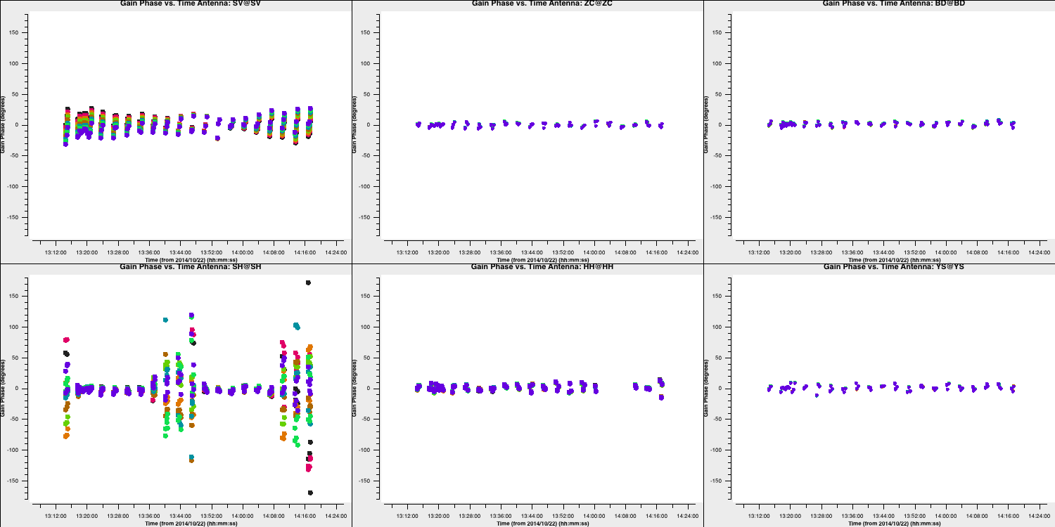
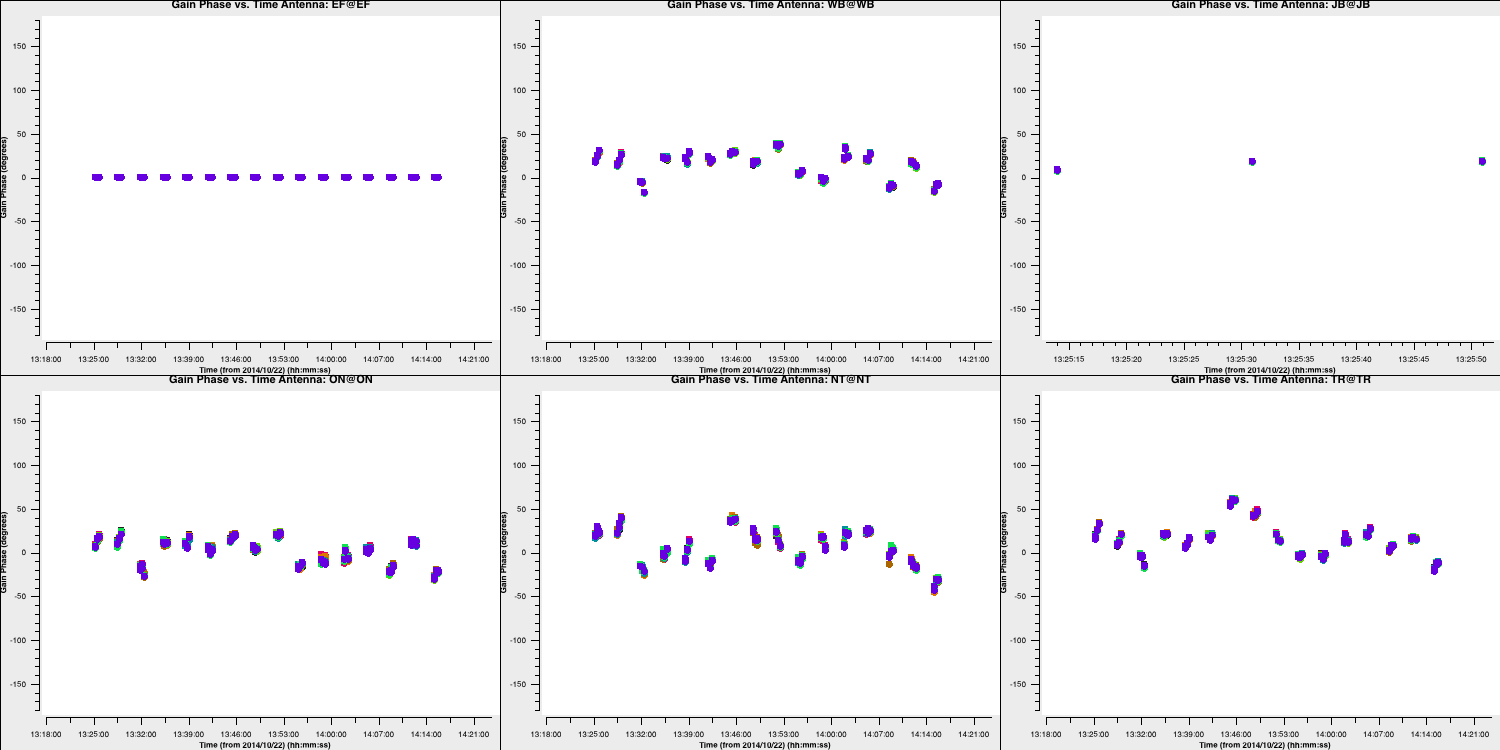
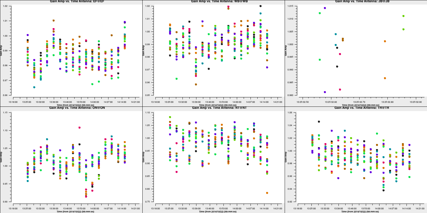
Also remember to fill in the plotms task. After doing that, execute step 4, and you should receive solutions like this:

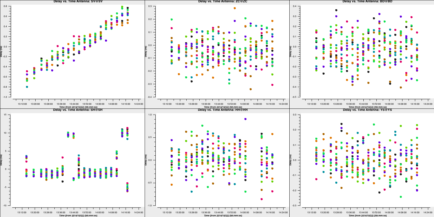
For most telescopes, the delays are nearly zero; therefore, the original fringe-fitting solutions were effective. In the case of Shenshen, we observe much larger corrections that vary across the spectral window and polarisations. These solutions appear promising and should address our delay issues. Let's apply these solutions and refine the phases next.

4C. Refining the phases

← back to top

By using these new delay solutions, we should now be able to derive corrections to the phases over time. Once again, we need to establish a solution interval.

• Using plotms, type the following into your CASA prompt:

default(plotms)
vis='1848+283_J1849+3024.ms'
xaxis='time'
yaxis='phase'
spw='1'
field='1848+283'
correlation='RR,LL'
avgchannel='32'
antenna='EF&*'
iteraxis='baseline'
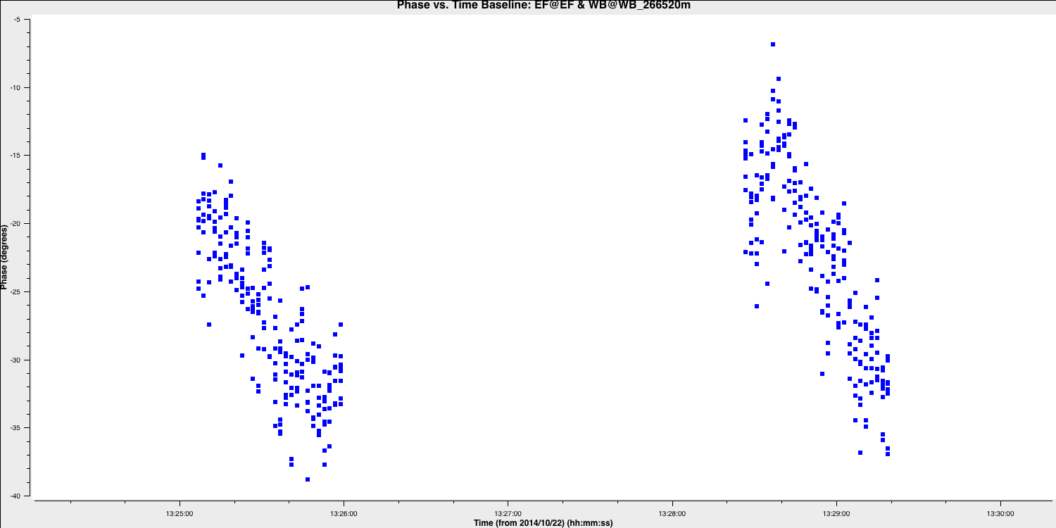
plotms()

You should see that the phases are close to zero for most baselines; however, some still exhibit large deviations (e.g., Shenshen; see plot below). Ideally, we want a solution interval that provides at least two data points per scan, allowing linear interpolation to track effectively between scans and enabling us to apply more accurate phase solutions to the target field. A 20s solution interval can yield three solutions per scan, with sufficient S/N to achieve good solutions.

Note that the plot above shows all spectral windows colourised by spw.

• Considering this, refer to step 5 in the skeleton script.

### 5) Refine phase calibration
mystep = 5

if(mystep in thesteps):
	print('Step ', mystep, step_title[mystep])

	# Gain calibration of phases only
	os.system('rm -r '+phscal+'_'+target+'.p')
	gaincal(vis=phscal+'_'+target+'.ms',
			field=phscal,
			caltable=phscal+'_'+target+'.p',
			corrdepflags=True,
			solint='xxx',
			refant='xxx',
			gaintype='xxx',
			minblperant='xxx',
			calmode='xxx',
			gaintable=['xxx'],
			parang='xxx')

	plotms(vis=phscal+'_'+target+'.p',
		   gridrows=2,
		   gridcols=3,
		   plotrange=[0,0,-180,180],
		   yaxis='xxx',
		   xaxis='xxx',
		   iteraxis='xxx',
		   coloraxis='xxx')

Many parameters should remain consistent with the delay calibration, but here are some additional pointers for the parameters that require adjustment. Note that we set the y-axis plot range from -180 to 180 degrees to visualise the scale of the phase corrections.

• gaintype - once more, review the help documentation to locate the appropriate code for gain / phase calibration.
• calmode - refer to the help documents to find the code for phase-only calibration.
• gaintable - set this so that the delay solutions are applied on the fly.
• minblperant - We want to determine closure quantities to ensure baseline-based errors are not corrected (the visibilities will be overly constrained by the model). Therefore, for phases, we need three baselines per antenna and four for amplitudes.

• If you are happy, execute step 5 and you should see the following phase solutions.

You can see that for most baselines the corrections are small; however, for the Shenshen telescope, these corrections are quite significant. To determine if these corrections improve our data, we need to apply them to the data.

4D. Apply corrections to the phase calibrator

← back to top

Let's apply the solutions using applycal.

• Take a look at step 6 and the inputs to the task applycal.

# 6) Apply delay and phases
mystep = 6

if(mystep in thesteps):
	print('Step ', mystep, step_title[mystep])

	# Apply these solutions to the phase cal
	applycal(vis=phscal+'_'+target+'.ms',
			 field='xxx',
			 gaintable=['xxx','xxx'],
			 gainfield=['xxx','xxx'],
			 interp=['xx','xx'],
			 applymode='xxx',
			 parang=False)

For this application of the solutions, we just want to calibrate the phase calibrator to inspect how well the solutions improve the visibilities. Because of this, the interpolation mode is not too important; that is, nearest or linear are identical here. Since only a few solutions fail, the applymode option which flags data, is acceptable here.

• Set the parameters of step 6 and execute the task.
• Once complete, re-plot the plotms command from part C of this section to see the improvements. Remember to set ydatacolumn='corrected'.

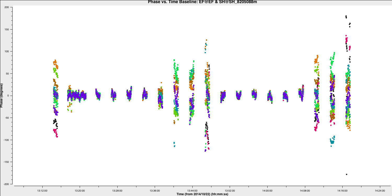
The plot below illustrates the improvement of the EF to SH baseline with these new delay and phase solutions applied. There are some erroneous data points that could be flagged; however, this will not significantly affect the final result.

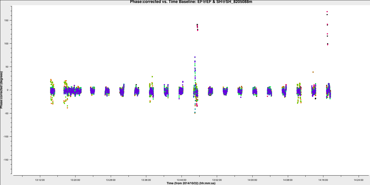
If you wish to flag the data, use the interactive flag tool and iterate over the SH baselines, flagging as you go along (use the previous plotms commands but set spw='' and antenna='SH&*')

5. Correct amplitude errors on the phase calibrator

5A. Re-image the phase calibrator

← back to top

With the corrections applied, we should image the phase calibrator again to create a better model for the next round of calibration.

• Refer to step 7 in the skeleton file. You will notice that we have now merged the deconvolution, the generation of the $\texttt{MODEL}$ column, and the image statistics into a single step. The parameters you enter should match those used previously.

### 7) Image phase calibrator again!
mystep = 7

if(mystep in thesteps):
	print('Step ', mystep, step_title[mystep])

	os.system('rm -r phasecal1p1.*')

	if mac==False:
		tclean(vis=phscal+'_'+target+'.ms',
			   imagename='phasecal1_p1',
			   stokes='pseudoI',
			   psfcutoff=0.5,
			   specmode='mfs',
			   threshold=0,
			   field='xxx',
			   imsize=['xxx','xxx'],
			   cell=['xxx'],
			   gridder='xxx',
			   deconvolver='xxx',
			   niter='xxx',
			   interactive=True)

	else:
		run_iclean(vis=phscal+'_'+target+'.ms',
				   imagename='phasecal1p1',
				   stokes='pseudoI',
				   specmode='mfs',
				   threshold=0,
				   field='xxx',
				   imsize=['xxx','xxx'],
				   cell=['xxx'],
				   gridder='xxx',
				   deconvolver='xxx',
				   niter='xxx')

	# Measure the signal-to-noise
	rms=imstat(imagename='phasecal1p1.image',
			   box='xxx,xxx,xxx,xxx')['rms'][0]
	peak=imstat(imagename='phasecal1p1.image',
			    box='xxx,xxx,xxx,xxx')['max'][0]

	ft(vis=phscal+'_'+target+'.ms',
	   field='xxx',
	   model='xxx',
	   usescratch=True)
	
	print('Peak %6.3f Jy/beam, rms %6.3f mJy/beam, S/N %6.0f' % (peak, rms*1e3, peak/rms))

Using the same boxes as in step 2, I obtained $S_\mathrm{p} = 1.274\,\mathrm{Jy\,beam^{-1}}$, $\sigma = 0.033 \,\mathrm{Jy\,beam^{-1}}$, and $\mathrm{S/N}= 39$. The improvement is quite modest because the phases were primarily calibrated by fringe-fitting. Only the Shenshen telescope, which was not adequately calibrated during fringe-fitting, received significant corrections, but Sheshan does not contribute significant sensitivity.

5B. Obtain amplitude solutions

← back to top

In the next step, we aim to use the improved model visibilities to adjust the amplitudes. As demonstrated in section 2A of this tutorial, where we plotted the amplitude versus uv distance, some amplitudes were mis-scaled compared to the model. This step will address that issue.

• Look at step 8.

### 8) Derive amplitude solutions
mystep = 8

if(mystep in thesteps):
	print('Step ', mystep, step_title[mystep])
	os.system('rm -rf'+phscal+'_'+target+'.ap')
	gaincal(vis=phscal+'_'+target+'.ms',
			caltable=phscal+'_'+target+'.ap',
			corrdepflags=True,
			field='xxx',
			solint='xxx',
			refant='xxx',
			solnorm='xxx',
			gaintype='xxx',
			minblperant='xxx',
			calmode='xxx',
			gaintable=['xxx','xxx'],
			gainfield=['xxx','xxx'],
			interp=['linear','linear'],
			parang=False)

	plotms(vis=phscal+'_'+target+'.ap',
		   gridrows=2,
		   gridcols=3,
		   yaxis='xxx',
		   xaxis='xxx',
		   iteraxis='antenna',
		   coloraxis='spw')

While most of these parameters can be the same as those used for the phase-only calibration, we need to change a few. Here are some hints for the ones that need to be changed.

• solint - solution interval. Most amplitude errors stem from the instrument; we expect this to vary more slowly than the phase errors coming from the atmosphere. Additionally, amplitude solutions require a higher S/N per solution interval. A good rule of thumb at GHz frequencies is the amplitude solution interval should be three times the phase-only solution interval.
• solnorm - this normalises the amplitude solutions, so the flux scale remains the same. Since we have already set this scale, we should set this to True.
• calmode - We want to pursue an amplitude and phase solution, as these tend to be more stable. Please check the task help for the correct code.
• gaintable and gaintable - remember that any calibration is done on the data column so we need to apply the other calibration tables on the fly.

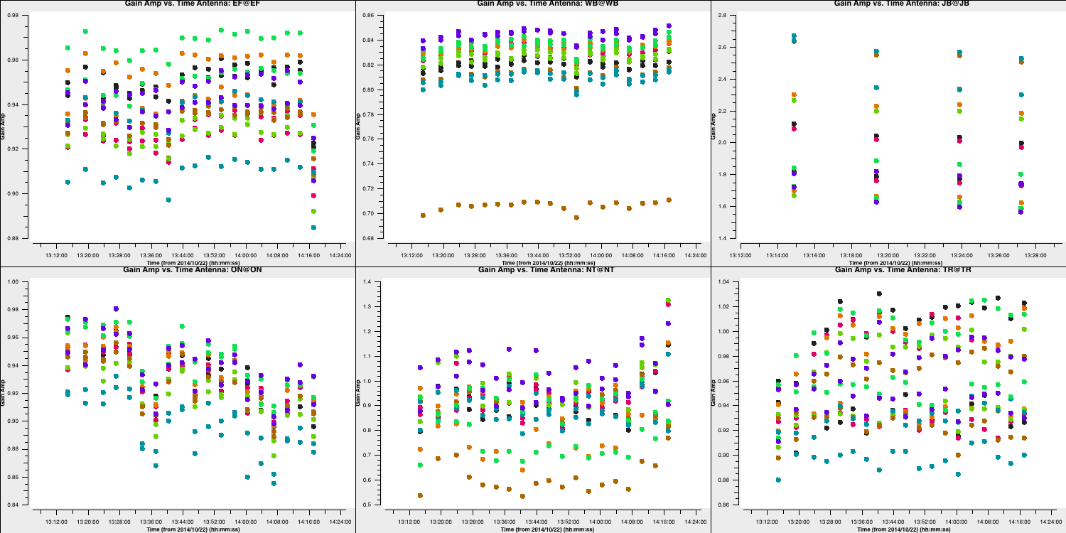
• If you are happy then put the parameters into both tasks and run step 8.

The plot below shows the amplitude solutions for each telescope and spw. You can see that for the majority of telescopes, the solutions are close to unity; hence, they were well calibrated by the $T_\mathrm{sys}$ measurements we used in part 1. However, some telescopes, such as Westerbork (Wb), are rescaled by this correction.

5C. Apply amplitude solutions

← back to top

Having derived and verified the amplitude solutions, we should apply them to the phase calibrator to investigate the improvements resulting from this calibration before applying the solutions to the target source.

• Look at step 9.

### 9) Apply all calibration to the phase calibrator
mystep = 9

if(mystep in thesteps):
	print('Step ', mystep, step_title[mystep])

	applycal(vis=phscal+'_'+target+'.ms',
			 field='xxx',
			 gaintable=['xxx','xxx','xxx'],
			 gainfield=['xxx','xxx','xxx'],
			 interp=['xxx','xxx','xxx'],
			 parang=False)

• Enter the parameters to apply the solutions to the phase calibrator only.
• Run step 9.

5D. Re-image phase calibrator with amplitude solutions applied

← back to top

To ensure that the solutions we have derived are suitable for application to the target, we should conduct a final imaging of the phase calibrator to verify that the calibration has not introduced many errors (i.e., non-Gaussian noise, stripes, or artifacts). This can also highlight some low-level RFI, which may appear as stripes in the image.

• Refer to step 10 and enter the parameters to execute tclean/run_iclean once more. Note that this time we do not need to use ft to input the model, as we should be finished with calibration.

### 10) Image phase calibrator for last time
mystep = 10

if(mystep in thesteps):
	print('Step ', mystep, step_title[mystep])
	os.system('rm -r phasecal1ap1.*')

	if mac==False:
		tclean(vis=phscal+'_'+target+'.ms',
			   imagename='phasecal1ap1',
			   stokes='pseudoI',
			   psfcutoff=0.5,
			   specmode='mfs',
			   threshold=0,
			   field='xx',
			   imsize=['xx','xx'],
			   cell=['xxx'],
			   gridder='standard',
			   deconvolver='xxx',
			   niter='xxx',
			   interactive=True)

	else:
		run_iclean(vis=phscal+'_'+target+'.ms',
				   imagename='phasecal1ap1',
				   stokes='pseudoI',
				   specmode='mfs',
				   threshold=0,
				   field='xx',
				   imsize=['xx','xx'],
				   cell=['xxx'],
				   gridder='standard',
				   deconvolver='xxx',
				   niter='xxx')

	# Measure the signal to noise
	rms=imstat(imagename='phasecal1ap1.image',
			   box='xxx,xxx,xxx,xxx')['rms'][0]
	peak=imstat(imagename='phasecal1ap1.image',
			   box='xxx,xxx,xxx,xxx')['max'][0]

	print('Peak %6.3f Jy/beam, rms %6.4f mJy/beam, S/N %6.0f' % (peak, rms*1e3, peak/rms))

When you open the image in imview/CARTA, you will find that the signal-to-noise ratio (S/N) of the image has dramatically increased. Using the same boxes as before, I managed to obtain $S_\mathrm{p}=1.407\,\mathrm{Jy\,beam^{-1}}$, $\sigma=0.5622\,\mathrm{mJy\,beam^{-1}}$, and so a $\mathrm{S/N}=2502$.

If we examine the amplitude and phase versus uv distance plots again, we can see that the discrepant amplitudes we observed have aligned, and only a very small proportion of the data remains miscalibrated. This bad data shouldn't significantly affect the results, but you can flag it if you wish.

5E. Apply solutions to the target

← back to top

Now that we are generally pleased with the calibration, we should apply these calibration solutions to the target source. Since the target scans are interleaved with the phase calibrator scans, we should consider the best interpolation scheme for this task. We didn't discuss this in much detail during part 1, but we will now.

In CASA, there are two main interpolation methods: nearest and linear. These methods are easy to understand. Nearest interpolation means that data will be corrected using the nearest data point in time and frequency space, whereas 'linear' will connect a line between the two data points surrounding the data you want to correct and use the linear solution at that location.

If the true solutions do not change rapidly or if the derived solutions are close to the data you wish to correct, then both interpolation schemes are similar. However, when the change is significant, a considerable difference can arise.

In the plot below, we illustrate a model phase change induced on the signal from a source by the atmosphere over a single antenna. Across the phase calibrator, we assume we track the phase perfectly (red lines); however, we must interpolate across the target scans (with the true phase changes in gray). As you can see, the errors (bottom panel) in the nearest interpolation (which are a step-wise model) are larger than those in the linear interpolation, especially when the phase changes are more severe across the target scan.

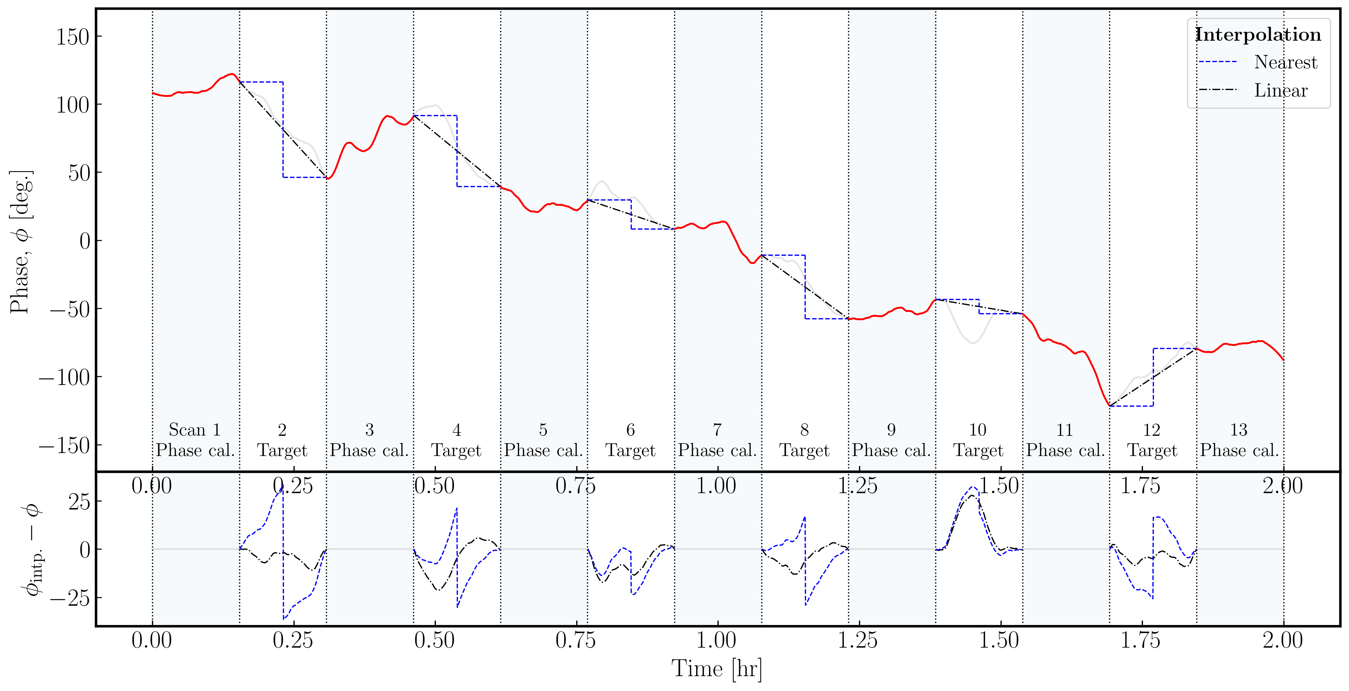
It is important to note that neither interpolation scheme can model any curvature (e.g., scan 10); therefore, the phase calibrator to target cycle times must be short enough for the phases, amplitudes, delays, and rates to be estimated linearly.

Either way, the optimal approach here is to use linear interpolation, as it typically tracks the target phase more effectively than nearest interpolation. Let's apply this knowledge to our refined solutions for the target.

• Refer to step 11 in the skeleton script.

### 11) Apply refined solutions to the target source
mystep = 11

if(mystep in thesteps):
	print('Step ', mystep, step_title[mystep])
	delmod(vis=phscal+'_'+target+'.ms')
	applycal(vis=phscal+'_'+target+'.ms',
			 field='xxx',
			 gaintable=['xxx','xxx','xxx'],
			 gainfield=['xxx','xxx','xxx'],
			 interp=['xxx','xxx','xxx'],
			 applymode='calonly',
			 parang=False)

• Input the parameters to apply all calibration to the target, and utilize linear interpolation to achieve this. Note that the applymode='calonly' is used to prevent unnecessary flagging of target data.
• Execute step 11.

5F. Split target

← back to top

The final step we need to take regarding the phase calibrator is to remove the calibrated target data and transfer it into a new measurement set. This will provide an intermediate backup data set, allowing us to derive further calibration using only the target source and not the phase calibrator.

• Refer to step 12 and enter the parameters to separate the target source data into a distinct measurement set.

### 12) Split target data out from the measurement set
mystep = 12

if(mystep in thesteps):
	print('Step ', mystep, step_title[mystep])
	os.system('rm -rf '+target+'.ms')
	os.system('rm -rf '+target+'.ms.flagversions')
	split(vis=phscal+'_'+target+'.ms',
		  outputvis=target+'.ms',
		  field='xxx',
		  correlation='xx,xx',
		  datacolumn='xxx')

Since we are not focused on polarisation in this tutorial, we will only output the parallel hand correlations (LL, RR) to reduce the measurement set size. Additionally, remember that we want to separate the calibrated data, so you need to set the datacolumn parameter.

• If you are happy, please execute step 12 to create the new measurement set named J1849+3024.ms. This will be the measurement set we will work on from now on.

6. Self calibration of target

6A. First target image

← back to top

With the solutions applied to the target field, we aim to assess it. Keep in mind that the phase solutions we derived for the phase calibrator will only be approximate because the telescopes observe slightly different areas of the sky. This indicates that we will encounter gain errors in our target field because the atmospheric conditions will be slightly different. In this section, we will replicate the procedure we used on the phase calibrator and perform self-calibration to eliminate these errors.

Firstly, we aim to create a model of the target field. This may not be point-like, so a reliable model is essential. Again, we just need to image the field and incorporate the model into the measurement set as before.

• Look at step 13.

### 13) First image of the target
mystep = 13

if(mystep in thesteps):
	print('Step ', mystep, step_title[mystep])
	
	os.system('rm -r target1phsref*')

	if mac==False:
		tclean(vis=target+'.ms',
			   imagename='target1phsref',
			   stokes='pseudoI',
			   psfcutoff=0.5,
			   specmode='mfs',
			   threshold=0,
			   imsize=['xxx','xxx'],
			   cell=['xxx'],
			   gridder='standard',
			   deconvolver='xxx',
			   niter='xxx',
			   interactive=True)

	else:
		run_iclean(vis=target+'.ms',
				   imagename='target1phsref',
				   stokes='pseudoI',
				   specmode='mfs',
				   threshold=0,
				   imsize=['xxx','xxx'],
				   cell=['xxx'],
				   gridder='standard',
				   deconvolver='xxx',
				   niter='xxx')

	ft(vis=target+'.ms',
	   model='target1phsref.model',
	   usescratch=True)

	# Measure the signal to noise
	rms=imstat(imagename='target1phsref.image',
			   box='xx,xx,xx,xx')['rms'][0]
	peak=imstat(imagename='target1phsref.image',
			   box='xx,xx,xx,xx')['max'][0]

	print('Peak %6.3f mJy/beam, rms %6.4f mJy/beam, S/N %6.0f' % (peak*1e3, rms*1e3, peak/rms))

• Input the parameters. You should be able to use similar parameters as those for the imaging of the phase calibrator. Also, note the change in the measurement set name used.
• The boxes for tracking the r.m.s. and peak should resemble those of the phase calibrator, provided you have used the same image size. However, make sure to verify that the same boxes are functioning correctly.
• If you are happy, execute step 13.

Using the same boxes as the phase calibrator I managed to obtain $S_p = 0.215\,\mathrm{Jy\,beam^{-1}}$, $\sigma=8.01\,\mathrm{mJy\,beam^{-1}}$, $\mathrm{S/N}= 27$. We should anticipate some improvements with the self-calibration iterations.

6B. Phase self-cal solution interval

← back to top

Whenever we perform self-calibration, we aim to conduct phase calibration first. This requires less signal-to-noise to obtain good solutions and poses less risk of making your visibilities resemble your model too closely. In self-calibration, we seek the most probable sky brightness distribution; therefore, an iterative approach guided by our model and the deconvolution process is the best option.

For this phase self-calibration, we need to derive an appropriate solution interval.

• Look at step 14 in the script.

### 14) Get phase solution interval for phase self-calibration
mystep = 14

if(mystep in thesteps):
	print('Step ', mystep, step_title[mystep])

	plotms(vis=target+'.ms',
		   xaxis='xxx',
		   yaxis='xxx',
		   correlation='xx',
		   antenna='xxx',
		   iteraxis='xxx',
		   avgtime='xx',
		   avgchannel='xx')

• Iterate through the baselines. An example is provided below for the Ef to Wb baseline, focusing on the LL correlation, spectral window zero, and the first couple of scans. You will notice some phase jumps across scans, along with general trends within the scans. A single scan per solution interval will only correct jumps between scans, so at least two are necessary to track changes within a scan.
• Now, we want to ensure we obtain sufficient S/N per solution, so use the avgtime parameter to determine if the averaged solutions reflect the phase trends rather than noise.
• Once you find an appropriate interval, write it down, and we will use it as your solution interval. I used 20 seconds because this provides three points with equal amounts of data per scan (since each scan is 1 minute).

6C. Derive phase self-cal solutions

← back to top

We now have our solution interval, so:

• Refer to step 15 and enter the parameters, including the solution interval obtained in the previous part of this step. We aim to derive phase only solutions.

### 15) Derive phase self-calibration solutions
mystep = 15

if(mystep in thesteps):
	print('Step ', mystep, step_title[mystep])

	os.system('rm -rf '+target+'.p')
	gaincal(vis=target+'.ms',
			caltable=target+'.p',
			corrdepflags=True,
			solint='xx',
			refant='xx',
			gaintype='xx',
			calmode='xx',
			parang=False)

	plotms(vis=target+'.p',
		   gridrows=2,
		   gridcols=3,
		   plotrange=[0,0,-180,180],
		   yaxis='xxx',
		   xaxis='xxx',
		   iteraxis='xxx',
		   coloraxis='xxx')

• If you are happy, run step 15.
• Remember to check the solutions and the logger to ensure that there are minimal failed solutions and that the solutions are sensible (like the ones below).

6D. Apply and image target again

← back to top

Now we will begin combining more tasks at once. In this part, we want to apply our phase self-calibration solutions, create another image, and then incorporate this model into the measurement set. Most of the parameters are the same; therefore, there will be minimal hints.

• Look at step 16.
• Input the parameters to apply the solutions and make a new image. We can use the same parameters as before.

### 16) Apply and image target again
mystep = 16

if(mystep in thesteps):
	print('Step ', mystep, step_title[mystep])
	applycal(vis=target+'.ms',
			 gaintable=[target+'.p'],
			 interp=['xx'],
			 applymode='calonly',
			 parang=False)

	os.system('rm -r target1p*')

	if mac==False:
		tclean(vis=target+'.ms',
			   imagename='target1p',
			   stokes='pseudoI',
			   psfcutoff=0.5,
			   gridmode='mfs',
			   threshold=0,
			   imsize=['xxx','xxx'],
			   cell=['xxx'],
			   gridder='standard',
			   deconvolver='clark',
			   niter='xxx',
			   interactive=True)

	else:
		run_iclean(vis=target+'.ms',
				   imagename='target1p',
				   stokes='pseudoI'
				   gridmode='mfs',
				   threshold=0,
				   imsize=['xxx','xxx'],
				   cell=['xxx'],
				   gridder='standard',
				   deconvolver='clark',
				   niter='xxx')

	ft(vis=target+'.ms',
	   model='xxx',
	   usescratch=True)

	# Measure the signal to noise
	rms=imstat(imagename='target1p.image',
			   box='xx,xx,xx,xx')['rms'][0]
	peak=imstat(imagename='target1p.image',
			   box='xx,xx,xx,xx')['max'][0]

	print('Peak %6.3f Jy/beam, rms %6.4f mJy/beam, S/N %6.0f' % (peak, rms*1e3, peak/rms))

• If you are happy with your inputs, then execute step 16.

You should find that the S/N of your source has increased a lot. I managed to get $S_p = 0.241\,\mathrm{Jy\,beam^{-1}}$, $\sigma=0.74\,\mathrm{mJy\,beam^{-1}}$, $\mathrm{S/N}= 325$. If it hasn't increased, then your phase solutions are probably bad and you should review the previous step.

6E. Inspect target structure

← back to top

As a brief aside, let's examine the structure of the target and the model we just derived. In this section, no inputs are needed, and you can simply run step 17. This will create the amp vs. uvwave plots for both the corrected data and the model.

In particular, one can see that along the west-east baselines, the source remains mostly unresolved (i.e., flat across uv space). However, on the long north-south baselines towards HH, the source is resolved. This is evident in the image, which shows a faint jet to the north-west! Before imaging routines were developed, this was the method radio astronomers used to derive source structure.

6F. Amplitude self-calibration

← back to top

With the phases now aligned, we want to correct any amplitude errors on our target source now that we have a large model S/N to work with. Remember from earlier, we aim to increase the S/N per solution interval, and a good rule of thumb is three times the phase-only solution interval.

• Look at step 18.

### 18) Derive amplitude solutions
mystep = 18
if(mystep in thesteps):
	print('Step ', mystep, step_title[mystep])

	os.system('rm -rf '+target+'.ap')

	gaincal(vis=target+'.ms',
			caltable=target+'.ap',
			corrdepflags=True,
			solint='xx',
			refant='xx',
			gaintype='xx',
			solnorm='xx',
			calmode='xx',
			gaintable=['xx'],
			parang=False)

	plotms(vis=target+'.ap',
		   gridrows=2,
		   gridcols=3,
		   yaxis='xxx',
		   xaxis='xxx',
		   iteraxis='xxx',
		   coloraxis='xxx')

	applycal(vis=target+'.ms',
			 gaintable=['xx','xx'],
			 applymode='calonly',
			 parang=False)

• Input the appropriate parameters to obtain amplitude and phase solutions, plot them, and apply them to the target source. Remember that we have already set the flux scale, so we should normalise the amplitude solutions.
• Once you are satisfied, execute step 18.
• Review the solutions to confirm their validity.

6G. Final imaging

← back to top

Now that we have corrected the amplitudes and phases, we want to image the source again to determine if the amplitude solutions have improved our signal-to-noise ratio (S/N). We do not expect a significant change from the amplitude self-calibration because most amplitude errors stem from the antenna itself, and this will largely be addressed by the phase calibrator's amplitude calibration.

• Look at step 19 and input the parameters into tclean/run_iclean and the imstat tasks.

### 19) Final imaging of target
mystep = 19
if(mystep in thesteps):
	print('Step ', mystep, step_title[mystep])

	os.system('rm -r target1ap.*')

	if mac==False:
		tclean(vis=target+'.ms',
			   imagename='target1ap',
			   stokes='pseudoI',
			   psfcutoff=0.5,
			   specmode='mfs',
			   threshold=0,
			   imsize=['xx','xx'],
			   cell=['xx'],
			   gridder='standard',
			   deconvolver='clark',
			   niter='xx',
			   interactive=True)

	else:
		run_iclean(vis=target+'.ms',
				   imagename='target1ap',
				   stokes='pseudoI',
				   specmode='mfs',
				   threshold=0,
				   imsize=['xx','xx'],
				   cell=['xx'],
				   gridder='standard',
				   deconvolver='clark',
				   niter='xx')

	ft(vis=target+'.ms',
	   model='target1ap.model',
	   usescratch=True)

	# Measure the signal to noise
	rms=imstat(imagename='target1ap.image',
			   box='xx,xx,xx,xx')['rms'][0]
	peak=imstat(imagename='target1ap.image',
			   box='xx,xx,xx,xx')['max'][0]

	print('Peak %6.3f Jy/beam, rms %6.4f mJy/beam, S/N %6.0f' % (peak, rms*1e3, peak/rms))

• If you are happy, proceed with step 19. The last command generates the amp/phase versus $uv$ distance plots from earlier. The parameters for this have been set for you.

I managed to get a large increase of S/N to $S_p = 0.244\,\mathrm{Jy\,beam^{-1}}$, $\sigma=0.202\,\mathrm{mJy\,beam^{-1}}$, $\mathrm{S/N}= 1205$.

• Using imview/CARTA, open the first target image along with the self-calibrated images and observe how the self-calibration process has improved the image fidelity, particularly regarding the noise profile.

This concludes this section of the tutorial. You've created your first calibrated image of a target source and learnt how to structure a simple calibration script. If you'd like to continue using this data, here are a few suggestions for extensions.

• Experiment with different weightings, such as uniform and robust, to determine if you can resolve the jet structure displayed on the long N-S baselines.
• Continue self-calibrating with finer solution intervals to determine if you can enhance the S/N even further.

Otherwise, let's move on to part 3, where you will create your own calibration script from scratch and calibrate the other phase calibrator-target pair we separated in part 1.