
Part 1: Basic Calibration
Guidance for calibrating EVN data using CASA
This guide used the self-contained (not modular) CASA version 6.5.4/5 (depending on your operating system).
Important: Before starting, please ensure that the correct version is on your system. On the UNIX command line type casa --nogui to open CASA and look for the following line on the command line and ensure that the highlighted number is equal or larger than 6.5.4:
CASA 6.6.5.31 -- Common Astronomy Software Applications [6.6.5.31]
If you find a version less than 6.5.4, please inform the DARA trainer who can provide the newer version. However, if the version is correct, type exit to exit CASA.
For this workshop, you'll need approximately 20 GB of disk space, although you could manage with less by transferring earlier versions of these files to storage.
In the following three parts, we shall build up to making your own calibration scripts by performing the data reduction in three different ways with reducing amount of assistance in each part:
- In Part 1 (this page), we will work interactively to see what each parameter is for. This is used for the initial steps and calibration common to all sources.
- In Part 2, we will calibrate and image one phase-reference and target by entering parameters into a script (
NME_J1849.py). - Finally, in Part 3, you shall use the information learnt in the previous sections to generate your own calibration script
NME_3C345_skeleton.pyfor the other phase-reference - target pair.
Table of contents
- Data and supporting material
- The CASA environment
- Data preparation
- Data loading and inspection
- Fringe-fitting
- Bandpass calibration
- Apply calibration and split out phase-ref - target pairs
1. Data and supporting material
n14c3 is an EVN network monitoring experiment to see how well the EVN is performing. It contains two target-phase-reference pairs of bright sources (plus a 5th source, which we will not use). These data are contained in FITS-IDI files, which are output from the correlator. The following table shows the sources in these files we are going to use. Don't worry about knowing what these are going to be used for yet; we will get around to this.
| Field ID | Name | Position (J2000) | Role |
|---|---|---|---|
| 0 | J1640+3946 | 16h40m29.632770s +39d46m46.02836s | Phase calibrator |
| 1 | 3C345 | 16h42m58.809965s +39d48m36.99402s | Target |
| 2 | J1849+3024 | 18h49m20.103406s +30d24m14.23712s | Target |
| 3 | 1848+283 | 18h50m27.589825s +28d25m13.15523s | Phase calibrator |
| 4 | 2023+336 | 20h25m10.842114s +33d43m00.21435s | Not used |
J1849+3024 is also used as a bandpass calibrator because it is a bright, compact source with good data on all baselines. If you are reducing a new data set, you would check the suitability of the bandpass calibrator early on in the data reduction process.
For this part, you should have downloaded the tar bundle (EVN_continuum_pt1_casa6.tar.gz) using the link on the home page. With this in hand let's start:
- Make a directory called something you will remember, e.g. EVN, and work in it. (Do not do data reduction within the CASA installation).
- Copy the data and files you need to this directory and extract the various scripts using
tar.<path_to_files>is the original location of these files.
Important: anything within triangular brackets, i.e. <> means something for you to fill in, and anything after a # is a comment.
mkdir EVN
cd EVN
cp <path_to_files>/EVN_continuum_pt1_casa6.tar.gz .

tar -xvf EVN_continuum_pt1_casa6.tar.gz   # extract the additional material.
- Let's check that all the data is there and we are in the right place. Type
pwdinto the UNIX command line, and you should see something like<path_to_files>/EVN/returned (where the path is the location which is often the UNIX home). Now typelsinto the command line and you should find at least the following files:
- Raw visibility data (FITS-IDI files from the JIVE correlator).
n14c3_1_1.IDI1n14c3_1_1.IDI2- Gain curve and $T_\mathrm{sys}$ data file
n14c3.antab- Helper scripts by Mark Kettenis to generate CASA-compatible $T_\mathrm{sys}$ and gain curves from the
.antabtable. casavlbitools- Nb: this is a folder!- Flag command files. You can write these yourself, but to save time you can use this one.
flagSH.flagcmd- The complete python calibration script (
NME_all.py.tar.gz) if you get stuck or need to re-calibrate quickly!
2. The CASA environment
To start CASA, we enter the simple command casa into the UNIX command line and should come up with the following (barring subtle changes due to the operating system you use):
casa

optional configuration file not found, continuing CASA startup without it

IPython 8.26.0 -- An enhanced Interactive Python.

Using matplotlib backend: MacOSX
CASA 6.6.5.31 -- Common Astronomy Software Applications [6.6.5.31]

CASA <1>:
For those familiar to ipython, this should look similar. Using this prompt, we shall use the various tasks and functions within CASA to begin calibrating our data. In addition, you will see that there is another window opened when we initialised CASA. This is the logger. The logger should look something like this:
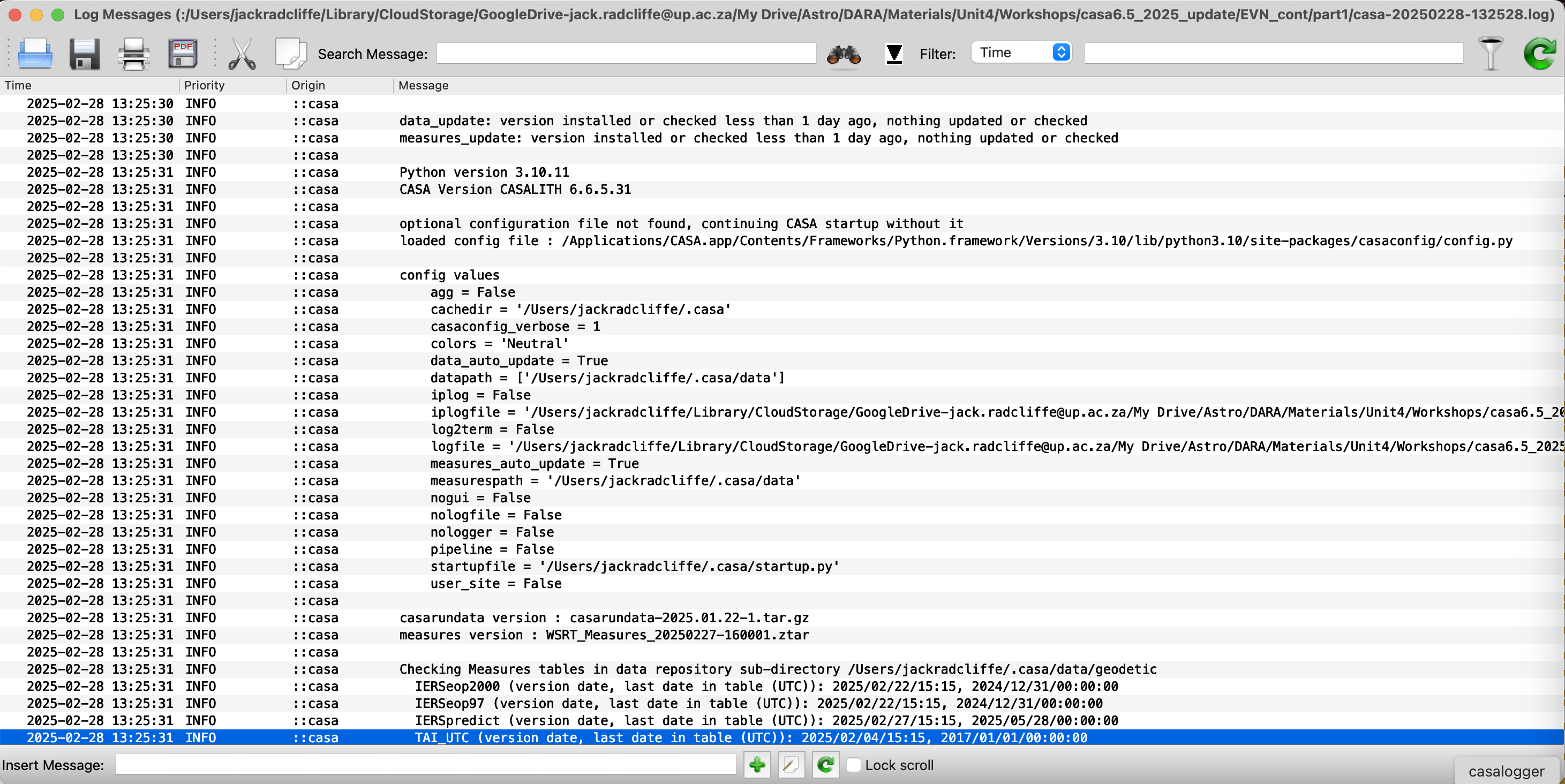
IMPORTANT: The logger will show the information on the tasks which have been executed, and if anything is erroneous or fails. It is vitally important to check this to evaluate the performance of the calibration. We will use this a lot during this tutorial.
3. Data preparation
Now we need to generate some a priori meta-data using the helper scripts contained in the casavlbitools module that was part of the tar bundle. The FITS-IDI files do not have any extra information on the individual antennas, such as the system temperatures ($T_\mathrm{sys}$), which provide the flux scaling for the observation, nor the gain curves, i.e., the difference in the effective sensitivity of the telescopes due to deformation of dishes because of gravity and differing atmospheric opacities with source elevation.
To start, we need to make the module available to CASA, therefore we need to put the casavlbitools folder in our path. Copy the following code and enter it into your CASA prompt:
import inspect, os, sys, json
sys.path.append(os.path.dirname(os.path.realpath('NME_all.py')))
This now allows us to import the various functions we need to generate the apriori meta-data. Firstly, we are going to attach the system temperature information to the FITS-IDI files using the append_tsys function. This needs to be done individually so input the following code into the command line:
from casavlbitools.fitsidi import append_tsys
append_tsys(antabfile='n14c3.antab', idifiles='n14c3_1_1.IDI1')
append_tsys(antabfile='n14c3.antab', idifiles='n14c3_1_1.IDI2')
The .antab file which contains the $T_\mathrm{sys}$ information and gain information is specified and then applied to the FITS-IDI files in turn. This may take a few minutes so have a coffee!
Once this is complete, we also need to extract the gain information for each antenna from the antab file. Again we use another function to do this namely append_gc. This will append the gaincurve information to the idifiles, which we shall convert to a gain curve later on (and explain what it does).
from casavlbitools.fitsidi import append_gc
append_gc(antabfile='n14c3.antab', idifile='n14c3_1_1.IDI1')
append_gc(antabfile='n14c3.antab', idifile='n14c3_1_1.IDI2')
It is worth noting that these pre-calibration steps are often different for other arrays. For example, the Very Long Baseline Array (VLBA) and newer (post-2022) EVN data comes with the gain curve and system temperatures already attached so the previous steps don't usually need to be used. In contrast, for Long Baseline Array (LBA) data you may need to make the antab table yourself and then attach to the idifiles. If you are unsure what needs to be done, contact a support scientist of the array that you're using. You won't mess up your data if you apply these accidentally twice.
4. Data loading and inspection
4A. Loading the data
Let's use our first task in CASA. We shall be using the importfitsidi task to change the FITS-IDI files (n14c3_1_1.IDI1 & n14c3_1_1.IDI2) we prepared earlier into a CASA compatible format called a measurement set.
Whenever we use a task in CASA (in interactive mode), it is always good practice to ensure that previous inputs are deleted since some inputs are shared across multiple tasks. In the CASA prompt, we can first initialize a task using default(<taskname>). For this purpose, we type default(importfitsidi) into the prompt instead.
With the task initialised, we need to set the inputs (explained later) for the task, i.e., what do we want the task to do? Typing inp into the prompt should return:
# importfitsidi -- Convert a FITS-IDI file to a CASA visibility data set
fitsidifile      = ['']  # Name(s) of input FITS-IDI file(s)
vis              = ''    # Name of output visibility file
constobsid       = False # If True, give constant obs ID==0 to the data from all input fitsidi files (False = separate obs id for each file)
scanreindexgap_s = 0.0   # Min time gap (seconds) between integrations to start a new scan
specframe        = 'GEO' # Spectral reference frame for all spectral windows in the output MS
So how do we interpret this? The labels to the left of the = are the inputs (e.g. fitsidifile, constobsid, specframe), and the values they are currently set to are to the right of the =. The default values indicate what type of input is required (e.g. [''] indicates a string array, while False denotes a Boolean, etc.). A brief description of each input follows the text after the hash symbol. To set the inputs, we use the syntax <input>=<value/array>. CASA assists here by colouring the input values red if the entry has the wrong data type (as is the case with the fitsidifile input currently) and blue if the input is set (i.e., non-default) and is of the correct type.
IMPORTANT: Remember that when using CASA, the help command is crucial. This command offers much more detail than the input command and can also provide examples of how to execute tasks. Try typing help(importfitsidi) in the command line. This should return something like:
Help on _importfitsidi in module casashell.private.importfitsidi object:

class _importfitsidi(builtins.object)
 |  importfitsidi ---- Convert a FITS-IDI file to a CASA visibility data set
 |
 |
 |  Convert a FITS-IDI file to a CASA visiblity data set.
 |  If several files are given, they will be concatenated into one MS.
 |
 |  --------- parameter descriptions ---------------------------------------------
 |
 |  fitsidifile      Name(s) of input FITS-IDI file(s)
 |                   Default: none (must be supplied)
 |
 |                      Examples:
 |                      fitsidifile='3C273XC1.IDI'
 |                      fitsidifile=['3C273XC1.IDI1','3C273XC1.IDI2']
 |  vis              Name of output visibility file
 |                   Default: none
 |
 |                      Example: outputvis='3C273XC1.ms'
 |  constobsid       If True, give constant obs ID==0 to the data from all
 |                   input fitsidi files (False = separate obs id for each file)
 |                   Default: False (new obs id for each input file)
 |                   Options: False|True
 |  scanreindexgap_s Min time gap (seconds) between integrations to start a
 |                   new scan
 |                   Default: 0. (no reindexing)
 |
 |                   If > 0., a new scan is started whenever the gap
 |                   between two integrations is > the given value
 |                   (seconds) or when a new field starts or when the
 |                   ARRAY_ID changes.
 |  specframe        This frame will be used to set the spectral reference
 |                   frame for all spectral windows in the output MS
 |                   Default: GEO (geocentric)
 |                   Options: GEO|TOPO|LSRK|BARY
 |
 |                   NOTE: if specframe is set to TOPO, the reference
 |                   location will be taken from the Observatories
 |                   table in the CASA data repository for the given
 |                   name of the observatory. You can edit that table
 |                   and add new rows.
You can type q to return to the CASA prompt. Note that you can also use the online CASA docs, which provide assistance for all of these tasks.
Ok, let's return to the importfitsidi task. We want to convert our FITS-IDI files to a CASA-compatible visibility file, known as a measurement set. When reviewing the inputs, we need to set at least the fitsidifile and vis inputs. We will also set the constobsid and scanreindexgap_s parameters, although these are not essential; they simply help to tidy up the data. Type the following inputs into your CASA prompt:
fitsidifile=['n14c3_1_1.IDI1','n14c3_1_1.IDI2']   # fits files to convert
vis='n14c3.ms'                             # output ms file name
constobsid=True                                   # data could be processed together
scanreindexgap_s=15                               # only separate scans if gap >15 sec (or source change)
IMPORTANT: After entering your inputs, always verify them before initiating the task. You don't want the task to mess up your data! Type inp() again, and you'll receive the following:
CASA <3>: inp
--------> inp()
#  importfitsidi :: Convert a FITS-IDI file to a CASA visibility data set
fitsidifile         = ['n14c3_1_1.IDI1', 'n14c3_1_1.IDI2'] #  Name(s) of input FITS-IDI file(s)
vis                 = 'n14c3.ms' #  Name of output visibility file (MS)
constobsid          =       True        #  If True, give constant obs ID==0 to the data from all input fitsidi files (False = separate obs id for each file)
scanreindexgap_s    =         15        #  min time gap (seconds) between integrations to start a new scan
specframe           =      'GEO'        #  spectral reference frame for all spectral windows in the output MS
As you can see, the inputs that have been set are now blue, and the fitsidifile input has turned blue, indicating that the data type is correct. If you are satisfied with the inputs, the task should be executed by typing either importfitsidi() or go()!
You will notice that the prompt has disappeared, and nothing can be typed into CASA until the task is finished. Take a look at the logger; this provides more information about the progress of the task, including what the task is doing and whether there are any errors associated with the inputs or the data sets.
Once the task is complete, you should find a new file named n14c3.ms. To view this file from within the CASA prompt, you can prepend an ! to the command to convert it into a UNIX command. For example, typing !ls should yield something similar to:
NME_all.py.tar.gz     flagSH.flagcmd      n14c3_1_1.IDI1
importfitsidi.last    n14c3_1_1.IDI2      casa-20250228-135515.log
n14c3.antab           casavlbitools       n14c3.ms
One of the most important aspects of data reduction is to understand your data! Without knowing what your data looks like and its quality, the resulting calibration can often be suboptimal. CASA provides many tools to assess and understand your data. The first, and one of the most essential of these, is the listobs task. This task outlines the structure of your data, such as the frequencies observed, the antennas involved, and the observing plan.
In the CASA prompt, initialise and run listobs. Remember to check the inputs and their functions using inp() before executing the task:
os.system('rm -rf n14c3.ms.listobs')  # note that this deletes the file that will be made with this task
default(listobs)
vis='n14c3.ms'
listfile='n14c3.ms.listobs'   # This makes a file with the listobs info.
listobs()
The command creates a file in the current working directory named n14c3.ms.listobs, which contains information about the measurement set. You can also set listfile="" to redirect this information to the logger instead. Try opening this file with your favourite text editor, such as gedit. Remember, placing a ! before the command allows you to run UNIX commands from CASA. Therefore, if you use gedit, the command to enter in the command line would be !gedit n14c3.ms.listobs.
What is included in this file?
- Scan listings. This shows the pattern of observations. Each scan is about 1 min and each individual integration about 2 sec.
  Date        Timerange (UTC)          Scan  FldId FieldName             nRows       SpwIds           Average Interval(s)
22-Oct-2014/12:00:00.0 - 12:04:00.0     1      1   3C345                 52800  [0,1,2,3,4,5,6,7]  [2, 2, 2, 2, 2, 2, 2, 2]
            12:06:00.0 - 12:10:00.0     2      1   3C345                 63360  [0,1,2,3,4,5,6,7]  [2, 2, 2, 2, 2, 2, 2, 2]
            12:12:00.0 - 12:13:00.0     3      1   3C345                 15840  [0,1,2,3,4,5,6,7]  [2, 2, 2, 2, 2, 2, 2, 2]
            12:13:40.0 - 12:14:40.0     4      1   3C345                 15840  [0,1,2,3,4,5,6,7]  [2, 2, 2, 2, 2, 2, 2, 2]
            12:15:20.0 - 12:16:20.0     5      0   J1640+3946            15840  [0,1,2,3,4,5,6,7]  [2, 2, 2, 2, 2, 2, 2, 2]
            12:17:00.0 - 12:18:00.0     6      1   3C345                 13200  [0,1,2,3,4,5,6,7]  [2, 2, 2, 2, 2, 2, 2, 2]
            12:18:40.0 - 12:19:40.0     7      0   J1640+3946            13200  [0,1,2,3,4,5,6,7]  [2, 2, 2, 2, 2, 2, 2, 2]
            12:20:20.0 - 12:21:20.0     8      1   3C345                 15840  [0,1,2,3,4,5,6,7]  [2, 2, 2, 2, 2, 2, 2, 2]
.......
- The names and positions of the observed sources. Note that two pairs of sources are close to each other in the sky. This will be important to remember when we start calibrating this data.
Fields: 5
ID   Code Name                RA               Decl           Epoch        nRows
0         J1640+3946          16:40:29.632770 +39.46.46.02836 J2000       254400
1         3C345               16:42:58.809965 +39.48.36.99402 J2000       383520
2         J1849+3024          18:49:20.103406 +30.24.14.23712 J2000       276480
3         1848+283            18:50:27.589825 +28.25.13.15523 J2000       388800
4         2023+336            20:25:10.842114 +33.43.00.21435 J2000       542880
- The frequency structure. There are eight spectral windows (or IFs), each consisting of 32 channels, and four polarisation products. We will only use the combined total intensity of RR and LL.
Spectral Windows:  (8 unique spectral windows and 1 unique polarization setups)
SpwID  Name   #Chans   Frame   Ch0(MHz)  ChanWid(kHz)  TotBW(kHz) CtrFreq(MHz)  Corrs
0      none      32    GEO    4926.990       500.000     16000.0   4934.7400   RR  RL  LR  LL
1      none      32    GEO    4942.490       500.000     16000.0   4950.2400   RR  RL  LR  LL
2      none      32    GEO    4958.990       500.000     16000.0   4966.7400   RR  RL  LR  LL
3      none      32    GEO    4974.490       500.000     16000.0   4982.2400   RR  RL  LR  LL
4      none      32    GEO    4990.990       500.000     16000.0   4998.7400   RR  RL  LR  LL
5      none      32    GEO    5006.490       500.000     16000.0   5014.2400   RR  RL  LR  LL
6      none      32    GEO    5022.990       500.000     16000.0   5030.7400   RR  RL  LR  LL
7      none      32    GEO    5038.490       500.000     16000.0   5046.2400   RR  RL  LR  LL
- The antennae participating in the observations. The offset from the array centre is zero since the absolute Earth-centred (geocentric) coordinates are given for each antenna.
Antennas: 12:
ID   Name  Station   Diam.    Long.         Lat.                Offset from array center (m)                ITRF Geocentric coordinates (m)
                                                                   East         North     Elevation               x               y               z
0    EF    EF        0.0  m   +006.53.01.0  +50.20.09.1          0.0000        0.0000  6365855.3595  4033947.234200   486990.818800  4900431.012900
1    WB    WB        0.0  m   +006.38.00.0  +52.43.48.0          0.0000        0.0000  6364640.6582  3828445.418100   445223.903400  5064921.723400
2    JB    JB        0.0  m   -002.18.30.9  +53.03.06.6         -0.0000        0.0000  6364633.4245  3822625.831700  -154105.346600  5086486.205800
3    ON    ON        0.0  m   +011.55.04.0  +57.13.05.3          0.0000        0.0000  6363057.6347  3370965.885800   711466.227900  5349664.219900
4    NT    NT        0.0  m   +014.59.20.6  +36.41.29.4          0.0000        0.0000  6370620.8444  4934562.806300  1321201.578200  3806484.762100
...
4B. Correct the antenna tables
As you may have noticed, the antenna information in the listobs output shows that the antennas have no diameters or axis offsets. In the future, this will be supplemented by a separate CASA task, but for now, we must insert it manually. While it's not crucial to remember, it might be easier to simply copy and paste the following commands into the CASA prompt:
# Copy these arrays of values (no line breaks in each array)
ants=  ['EF','WB','JB','ON','NT','TR','SV','ZC','BD','SH','HH','YS','JD']
diams= [100.0,25.0,75.0,25.0,32.0,32.0,32.0,32.0,32.0,25.0,24.0,40.0,25.0]
axoffs=[[0.013,4.95,0.,2.15,1.831,0.,-0.007,-0.008,-0.004,-0.002,6.692,2.005,0.]
,[0.,0.,0.,0.,0.,0.,0.,0.,0.,0.,0.,0.,0.]
,[0.,0.,0.,0.,0.,0.,0.,0.,0.,0.,0.,0.,0.]]

# Modify the antenna table
tb.open('n14c3.ms/ANTENNA', nomodify=False)
tb.putcol('DISH_DIAMETER', diams)
tb.putcol('OFFSET',axoffs)
tb.close()
Run a listobs (listobs(vis='n14c3.ms')) and check the logger to ensure that these have been updated accordingly! Note that we will use what we call a reference antenna later for calibration. This is typically chosen as either the most sensitive antenna in the array or the antenna with the largest number of short baselines. In this observation, the reference antenna will be the 100m diameter Effelsberg (EF) telescope.
4C. A priori calibration
If you recall, the append_tsys helper function was used to attach the system temperature information for each telescope to the FITS-IDI files. The system temperature is measured every few minutes, which compensates roughly for the varying signal levels from different sources, the effects of elevation, and other amplitude fluctuations. Each antenna has a distinctive response in terms of Kelvin of system temperature per Jy of flux, so $T_\mathrm{sys}$ is also used to scale the flux density, much like setting a temperature scale.
In CASA, calibration is conducted using calibration tables, which are then employed to modify the visibilities. To obtain our flux scaling, we therefore need to generate a system temperature calibration table using the task gencal. This task is designed to generate caltables from ancillary information found in the measurement set or in external files, and it can also be used to create manual calibration tables from scratch. The gencal task has a special function for generating $ T_\mathrm{sys}$ tables. To create these tables, we must input:
# In CASA
default(gencal)  # This reads the Tsys information appended to a ms
vis='n14c3.ms'
caltable='n14c3.tsys'
caltype='tsys'
uniform=False   #Set to False to get spw dependent Tsys extraction
gencal()
You will find that there is a new table named n14c3.tsys, which contains the flux scaling information.
IMPORTANT: A key factor in generating calibration tables is inspecting them for errant values that simply do not make sense. To inspect tables, we must use plotms. If you have previously used CASA (version $<$ 6.3), this functionality was provided by plotcal, but it has now been merged with plotms. When we initialise the task (remember to use default), there are many inputs to set. This task is very versatile and can be used to plot both calibration and visibilities, hence the plethora of inputs.
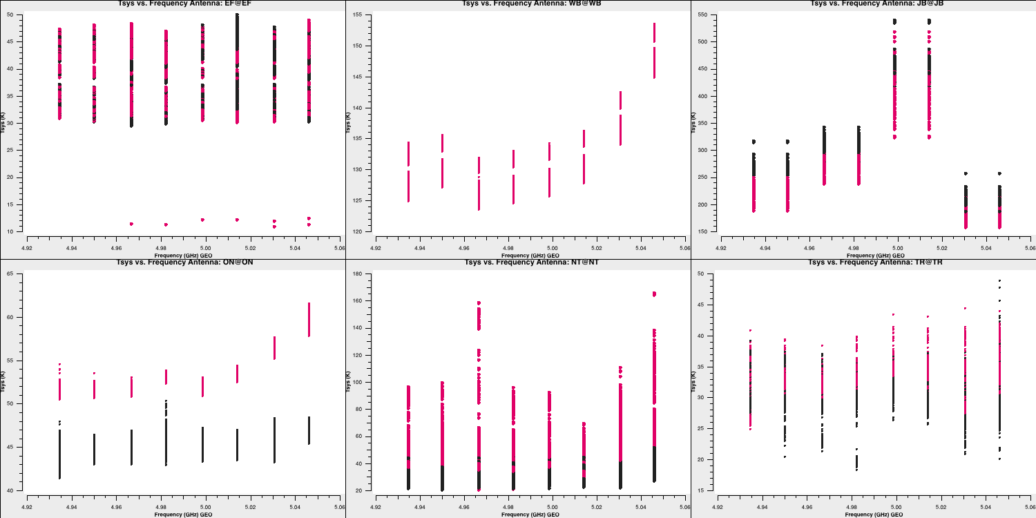
We need to set the $x$ and $y$ axes, as well as specify what each plot will iterate over. Firstly, we will plot $ T_\mathrm{sys}$ against frequency for each antenna. We will create multiple plots per page and colour our points by polarisation/correlation as well. Therefore, we will input the following:
default(plotms)
vis='n14c3.tsys'    # Name of the calibration file
xaxis='frequency'   # x-axis
yaxis='tsys'        # y-axis
gridrows=2          # number of rows to plot
gridcols=3          # number of columns so total plots = 6 = 2x3
coloraxis='corr'    # colour points by polarisation
iteraxis='antenna'  # iterate over the antennae (i.e. each plot is different antenna!)
plotms()
This should give an output similar to:
Note that the green arrows in the GUI can be used to iterate through the remaining antennae. We can also see how the $T_\mathrm{sys}$ varies over time! Most parameters are already set from the last run of plotms, so we can simply write (and remember to check the inputs before running!):
xaxis='time'
inp()
plotms()
This should generate a plot similar to:
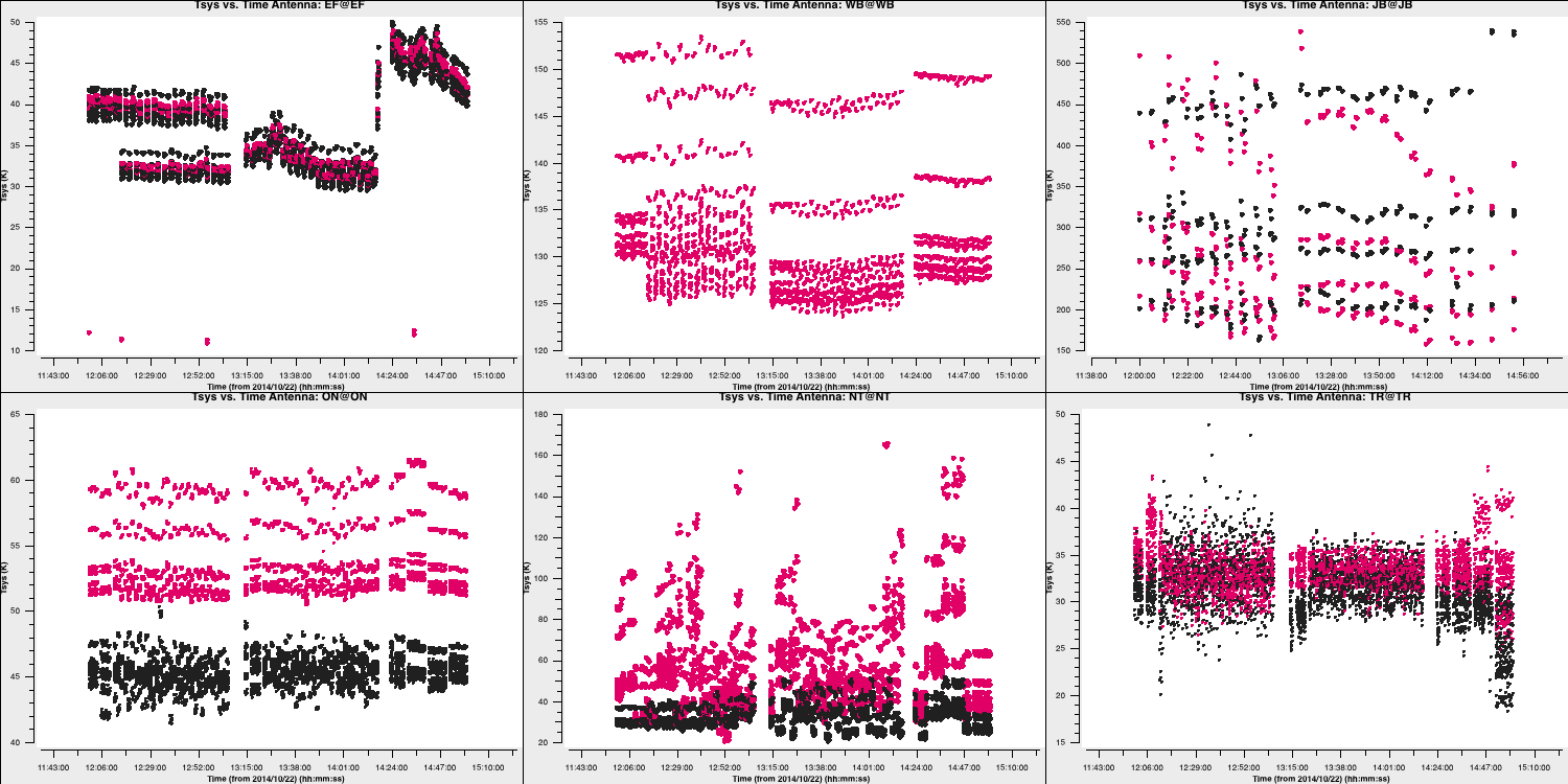
Three antennas lack $T_\mathrm{sys}$ measurements; however, in the next step, we will generate the gain curve table. This table provides the scaled gain-elevation correction, which adjusts the visibility amplitudes to the sensitivity of the dish, although it does not account for weather or source contributions. Again, we use gencal to accomplish this, which uses the gain information that we appended to the fitsidifiles earlier:
# In CASA
default(gencal)
vis="n14c3.ms"
caltable= "n14c3.gcal" ## Name of output gain curve cal. table
caltype="gc"           ## Special caltype for gaincurves
gencal()
4D. Inspect and flag data
One of the most important aspects of radio interferometric data reduction is identifying and removing bad data. As you will see in the lectures, often this bad data is due to Radio Frequency Interference (RFI) from satellites and mobile phones; however, sometimes it can stem from various other factors, such as correlation errors or antennas being off source. While it sounds tedious, the effects of bad data can be significant if ignored; therefore, careful extraction and removal of bad data is of paramount importance. In this sub-section, we shall inspect our visibilities and attempt to flag and remove bad data.
- To begin, we will remove the autocorrelations, as they are not useful for continuum interferometric observations. Occasionally, VLBI observations will use these measurements to obtain a scalar bandpass correction, but we will not do this here. To achieve this, we use the manual flagging task called
flagdata. - Let us review the inputs. To flag all of the autocorrelations, we simply leave everything at default (i.e., all data is selected) and set the
autocorrparameter to True.
# In CASA
default(flagdata)
vis='n14c3.ms'
mode='manual'
autocorr=True

flagdata()
- Next, we can see which telescopes are involved and their positions relative to each other by using the CASA task
plotants.
# In CASA
default(plotants)
vis='n14c3.ms'

plotants()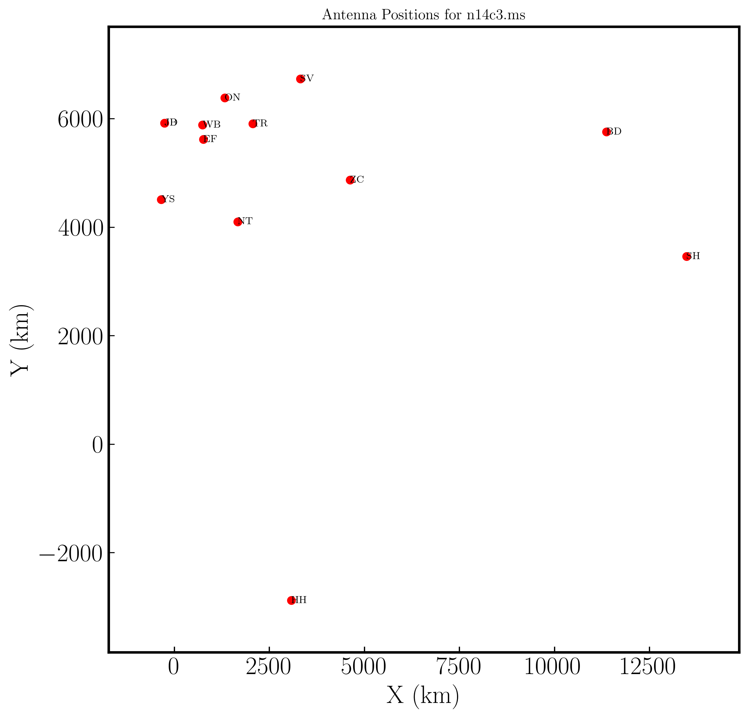
- To inspect data quality, we will use the task
plotmsagain to identify bad data. We begin by examining a bright source, which makes it easier to distinguish between good and bad data. Remember, theplotmstask is quite complex (refer to the task inputs) and can take some time to understand. We will first analyse the frequency axes (so we can average the time axes!) and then examine the baselines to the most sensitive telescope, which is the 100m Effelsberg dish.
# In CASA
default(plotms)
vis='n14c3.ms'
xaxis='frequency'
yaxis='amp'
field='1848+283'        # The phase-cal/bandpass cal
avgtime='3600'          # Will only average within scans unless additionally told to average scans too
antenna='EF&*'          # Plot all baselines to the largest and most sensitive antenna
correlation='RR,LL'     # Only plot the parallel hands; the cross hands are fainter (and we won't be using them).
coloraxis='antenna2'

plotms()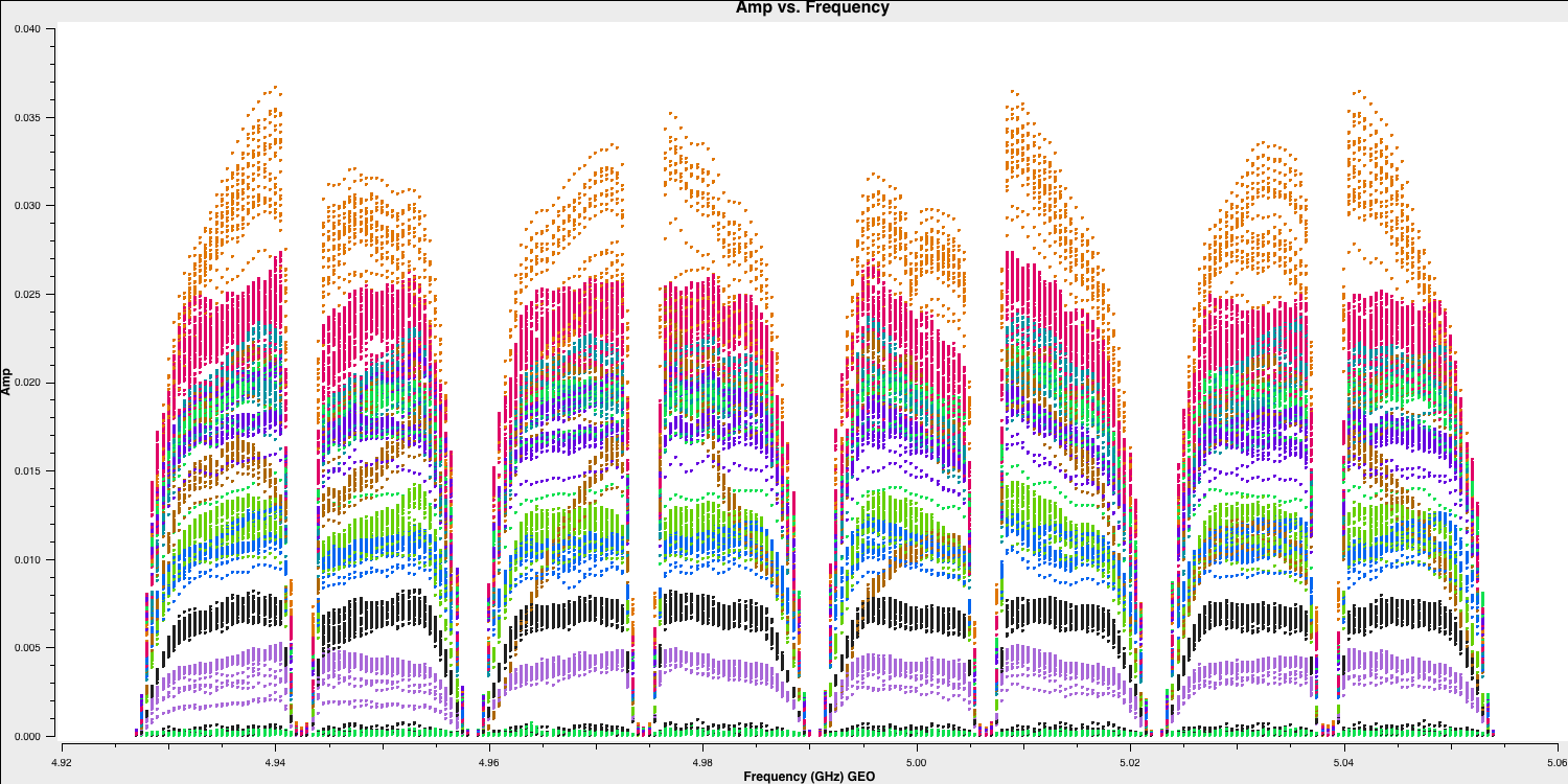
- You can interactively change the plot in plotms.
- There are eight spectral windows that are visible; the edges have low amplitudes due to poor sensitivity, and some data points are all at zero.
- Zoom in (using
 ) and use select to highlight bad data (
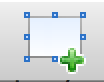 ), then use locate (
 ) to see which antenna it is associated with.
 - You should notice that this mostly pertains to antenna SV (Svetloe; dark green in this plot).
IMPORTANT: Before flagging more, remember to back up the current flags. Do this anytime you think you might change your mind about flagging. Use a different version name each time and make a note of it (the CASA task flagdata can create an automatic backup, but it will not have a memorable name). The backups for this data set are stored in n14c3.ms.flagversions. We will now back up the flags for this data set using the task flagmanager. This same task can also be used to revert to old flags.
# In CASA
default(flagmanager)
vis='n14c3.ms'
mode='save'           # This mode saves the current flags, use the mode restore to revert to old flagging versions
versionname='preSVandEndChans'  # This is the version name, you can see all version names in flagversions by using mode='list'
flagmanager()
- We should investigate Svetloe further to determine where the issues are originating. Returning to our plotms GUI, if we plot all baselines to Svetloe (by modifying the antenna parameter in the Data tab of the GUI to
SV&*), we can observe that there is some data on certain baselines. Next, we want to see if the issue is limited to specific baselines or affects the entire antenna. By changing the coloration (Display $\rightarrow$ Colorize = corr), we obtain the following:
- By using the locate function again, we observe that this is all related to the right-hand circular correlation (RR). With this knowledge, we can flag the correlation using the
flagdatatask that we used earlier.
# In CASA
default(flagdata)
vis='n14c3.ms'
correlation='RR'
mode='manual'
antenna='SV'
go()
If you have the plotms GUI still open, you can click reload and plot to see that the data has been removed, or you can run tget plotms and type go to execute the exact plotms parameters you used last time.
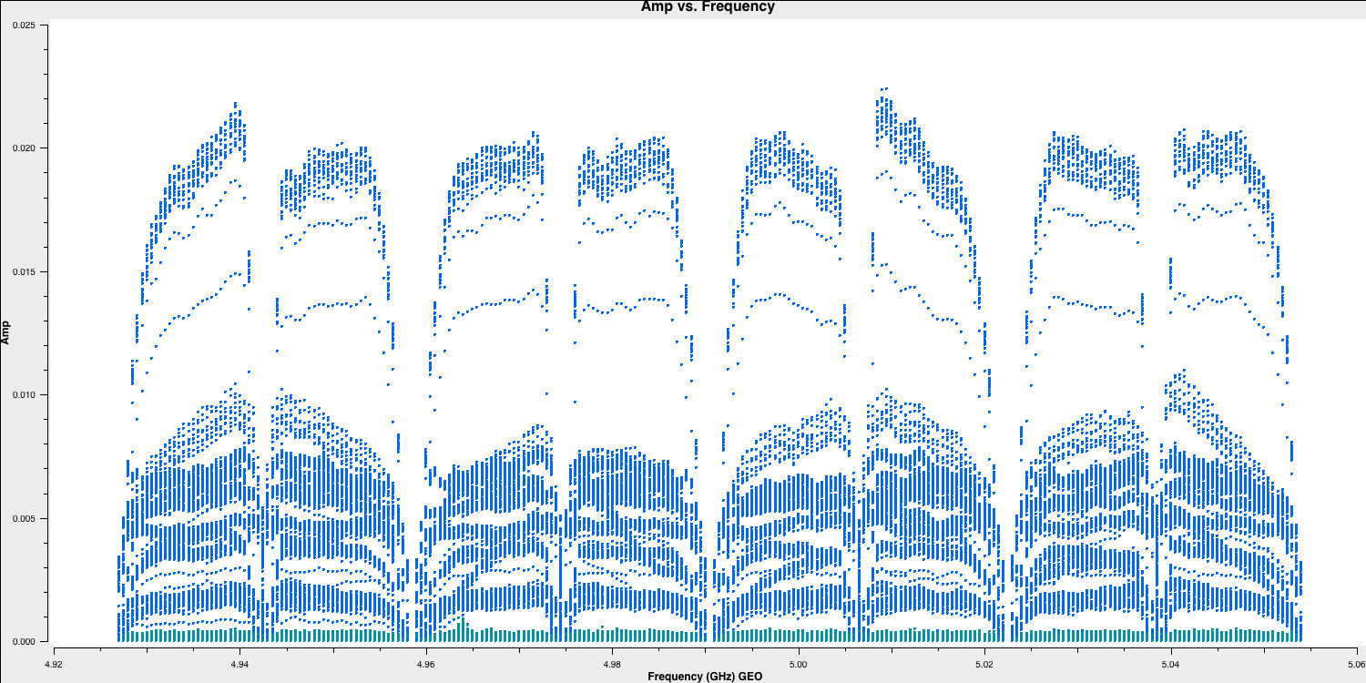
- Next, we should re-inspect the data for any additional corrupted entries. Plot the most sensitive baseline to visualise the end channels more clearly and identify which fall below approximately half of the maximum amplitude. These can cause issues later if not flagged and contribute little to the final image sensitivity.
# In CASA
default(plotms)
vis='n14c3.ms'
xaxis='channel'
yaxis='amp'
field='1848+283'        # The phase-cal/bandpass cal
avgtime='3600'          # Will only average within scans unless additionally told to average scans too
antenna='EF&JB'          # Plot the baseline of largest and most sensitive antennas
correlation='RR,LL'     # Only plot the parallel hands; the cross hands are fainter (and we won't be using them).
iteraxis='spw'

plotms()
- Use the arrows at the bottom of
plotmsto scroll through the spw (which should correspond to the subplots shown above). Odd and even spws behave differently, but there is no need to spend too much time on this, as the suggested channels to flag are provided here for time-saving purposes:
# In CASA
default(flagdata)
vis='n14c3.ms'
mode='manual'
spw='0:0~5;29~31,2:0~5;29~31,4:0~5;29~31,6:0~5;29~31,1:0~2;27~31,3:0~2;27~31,5:0~2;27~31,7:0~2;27~31'

flagdata()
We can check if this has worked by pressing reload in the plotms window and plotting it again. These edge channels should now be gone.
- Next, we will examine amplitude versus time, now averaging in frequency.
# In CASA
default(plotms)
vis='n14c3.ms'
xaxis='time'
yaxis='amp'
field='1848+283'
spw='0~7:13~20'        # Average a few central channels where the response is stable
avgchannel='8'
antenna='EF&*'
correlation='RR,LL'
coloraxis='baseline'

plotms()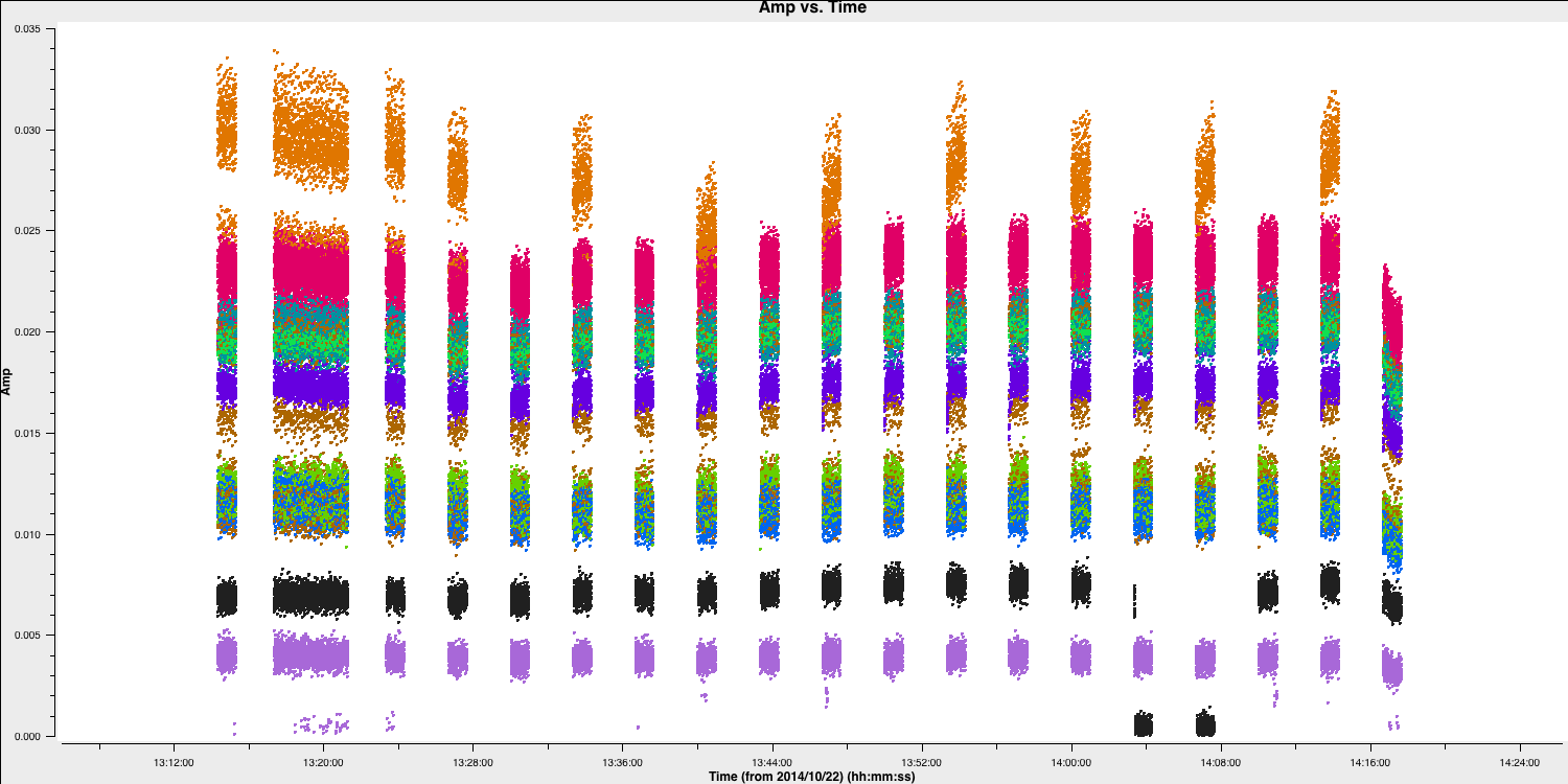
- Note that sometimes the first one or two integrations of certain scans may be poor (low amplitudes). There is a specific
flagdatamode for this called "quack". For the sake of time, we will assume that all sources are affected.
# In CASA
default(flagdata)
vis='n14c3.ms'
mode='quack'
quackinterval = 5     # 5 seconds, or just over 2 integrations

flagdata()
- Now review each baseline to identify any remaining bad data (enter
iteration='baseline'and reloadplotms). This has already been noted, so avoid spending too much time on it; just ensure you understand how to identify and record bad data. There is more than one flawed scan on HH, and since we are plotting the phase calibrator, it is likely that the target in between was affected. Please plot this.
# In CASA
default(plotms)

vis='n14c3.ms'
xaxis='time'
yaxis='amp'
scan='60~70'            # a few scans including the bad data; plot all fields in this time range
spw='0~7:13~20'
avgchannel='8'
antenna='EF&HH'         # just the relevant baseline
correlation='RR,LL'
coloraxis='field'       # distinguish sources

plotms()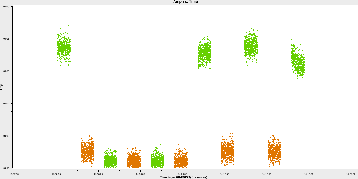
- Flag the scans when the target (shown in orange in the plot here) reaches zero. For your convenience, we have included the commands here.
# In CASA
default(flagdata)
vis='n14c3.ms'
antenna='HH'
mode='manual'
scan='62~65'

flagdata()
- Check that these have been removed by reloading plotms. Next, let's inspect the next most distant antenna, Sheshan (SH).
# In CASA
default(plotms)

vis='n14c3.ms'
xaxis='time'
yaxis='amp'
field='1848+283'
spw='0~7:13~20'
avgchannel='8'
antenna='EF&SH'         # just the relevant baseline
correlation='RR,LL'
coloraxis='spw'         # distinguish spw

plotms()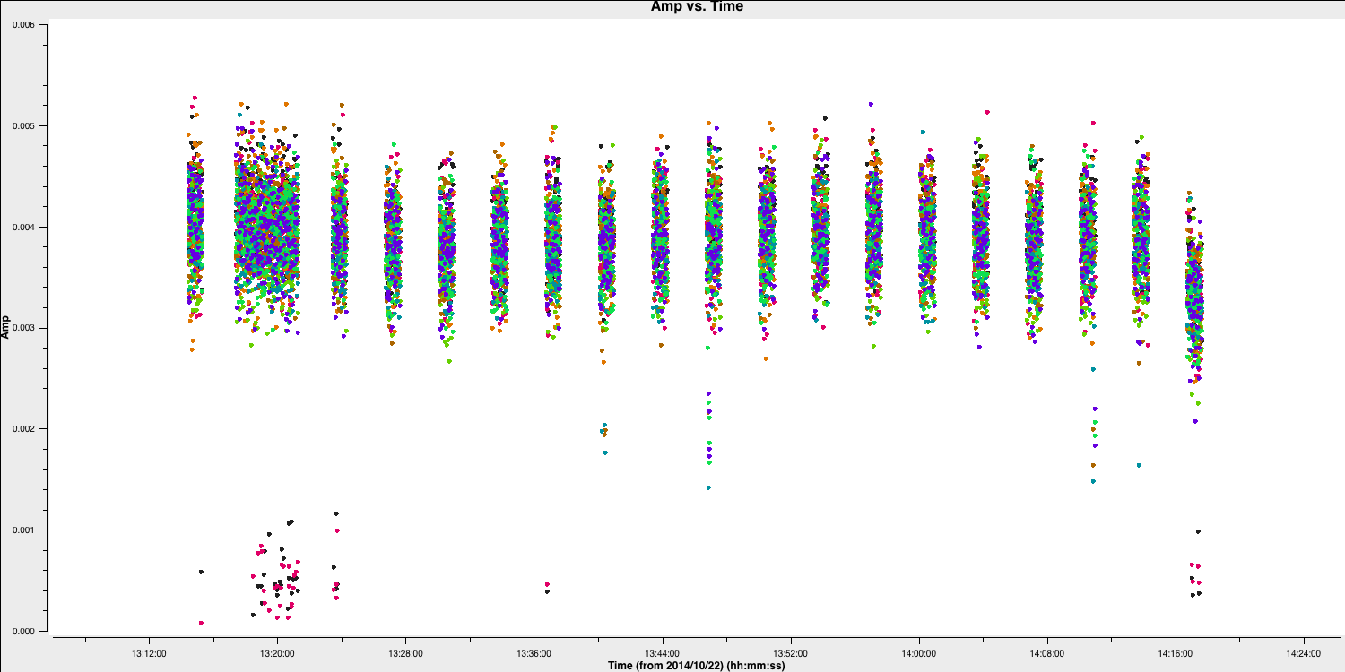
There are many short, problematic periods, some of which only affect certain spw. The easiest way to cope with this is to create a flag list. Identify antennas/spw/times, adding 1s to the start and end of each flagging period. They are all shorter than one scan, so the same flags aren't applied to the target, but later, we will look for similar bad data on the target.
- Review the flag list file (
flagSH.flagcmd) by opening it in a text editor and cross-checking that these entered values are affected. Typically, you will build this file yourself as different datasets will have different issues impacting it. However, this is often one of the most time-consuming parts of data reduction, so we have provided the answers to save time. - If you are happy, then we will use this file to automatically flag those channels specified in the file:
# In CASA
default(flagdata)
vis='n14c3.ms'
mode='list'
inpfile='flagSH.flagcmd'

flagdata()
Let's reinspect these data to check that the bad data are all gone:
# In CASA
default(plotms)
vis='n14c3.ms'
xaxis='time'
yaxis='amp'
field='1848+283'
spw='0~7:13~20'
avgchannel='8'
antenna='EF&*'
coloraxis='corr'
correlation='RR,LL'

plotms()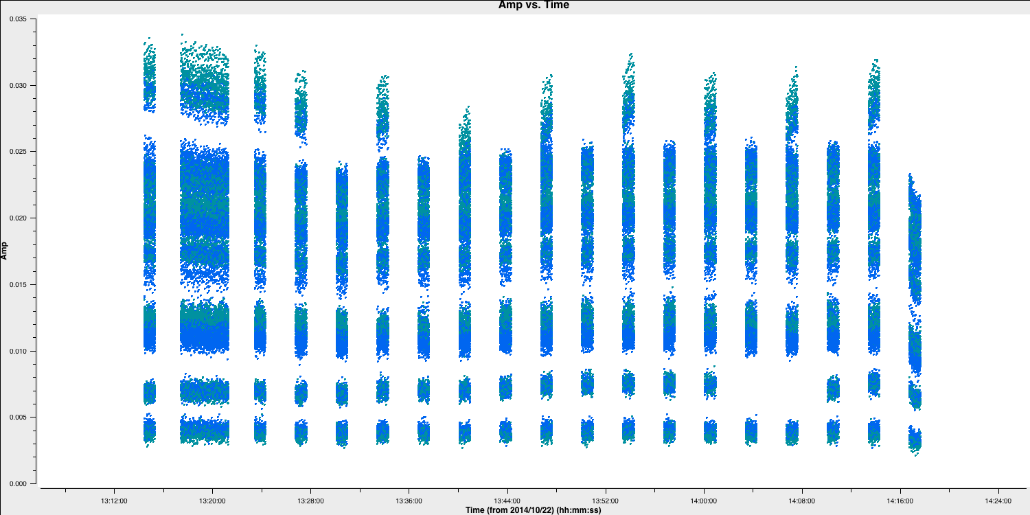
Great, these data looks clean! We can finally begin to calibrate these data!
5. Fringe fitting
Now that all the data has been cleaned up, we can begin to consider calibrating this data. As you may remember from the accompanying lectures, the wavefronts arriving at two different telescopes from a single source arrive at different times; one signal is delayed relative to the other. This is illustrated by the $D\sin(\theta)$ term in the two-element interferometer shown below:
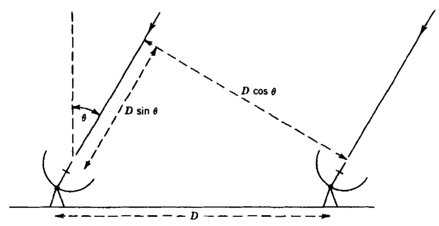
The actual delay term, $\tau_\mathrm{obs} = (D/c)\sin(\theta)$, changes over time because the source position relative to the baseline varies. This means that the interferometer phase ($\phi=2\pi\nu\tau_\mathrm{obs}$) also changes with time, leading to what we refer to as fringe rates. The correlator corrects for $\tau_\mathrm{obs}$ using a model that is often adequate for a short baseline, but, for VLBI, there are often residual errors present after the correction.
These residual phase, delay, and rate errors are mainly due to atmospheric fluctuations and residuals from the geometric delay compensation by the correlator. Since the phase ($\phi$) is related to the delay ($\tau_\mathrm{obs}$), the phase error will depend on the delay error! To solve for the phase error ($\Delta\phi$), we assume a linear phase model for each antenna, $$\Delta\phi(t,\nu)=\phi_{0}(t,\nu) + \left(\frac{\partial\phi}{\partial\nu}\Delta\nu + \frac{\partial\phi}{\partial t}\Delta t\right),$$ where $\phi_{0}$ is the phase error at a time and frequency, $\frac{\partial\phi}{\partial\nu}\Delta\nu$ is the delay and $\frac{\partial\phi}{\partial t}\Delta t$ is the rate term. Therefore for a baseline with antennae $i$ and $j$, the relative phase error, $\Delta\phi(t,\nu)_{ij}$ can be modelled as, $$\Delta\phi(t,\nu)_{ij}=\phi_{0i} - \phi_{0j} + \left(\left[\frac{\partial\phi_i}{\partial\nu}-\frac{\partial\phi_j}{\partial\nu}\right]\Delta\nu + \left[\frac{\partial\phi_i}{\partial t} - \frac{\partial\phi_j}{\partial t}\right]\Delta t\right).$$ In the following section, we will attempt to solve this equation by using all the baselines to estimate the phase delay and rates relative to a reference antenna. Remember that the interferometer is sensitive to differences; therefore, the relative phases, delays, and rates need to be corrected, not the absolute value!
5A. Instrumental delays
Some of the errors in the aforementioned equation originate from instrumental effects. In systems where different spectral windows have different electronics, the signal chain at the telescope itself can introduce delays. This can be thought of as the signal at different frequencies travelling different lengths of cable. These delays are mostly constant across the observation time (the residuals are corrected later); therefore, we can use a small chunk of data to estimate these (on timescales < the change of delay induced by the atmosphere). Let's plot a small chunk of data to illustrate these delays:
# In CASA
default(plotms)
vis='n14c3.ms'
xaxis='frequency'
yaxis='phase'
ydatacolumn='data'
antenna='EF'
correlation='LL'
coloraxis='baseline'
timerange='13:53:20.0~13:54:20.0'
averagedata=True
avgtime='120'
plotms()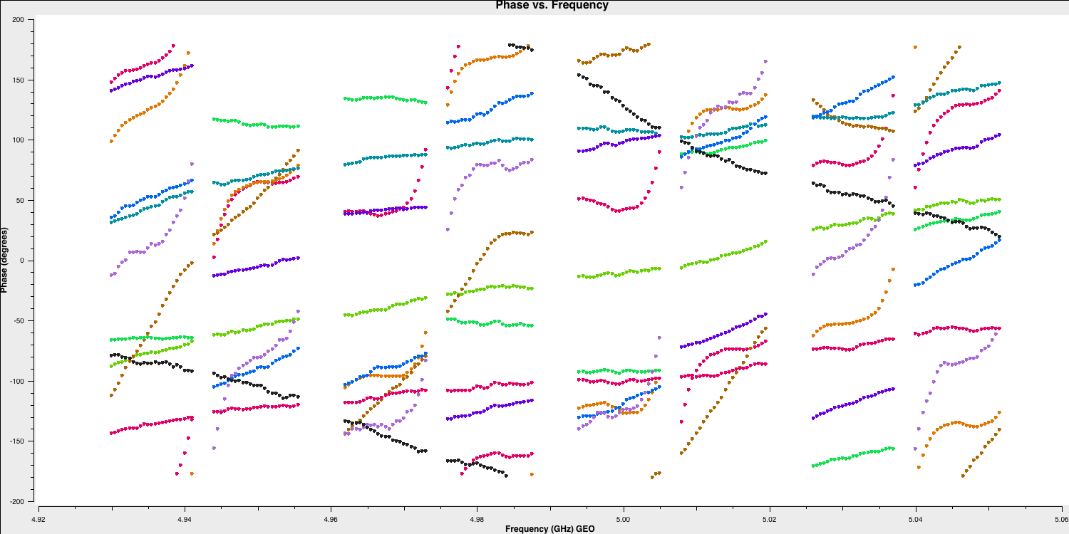
You can observe that the instrumental delays appear as jumps in phase between the spectral windows. If you pay attention, we are using a small time range (approximately 4 minutes) on a bright source (1848+283) because, to characterise these jumps, we require a high signal-to-noise ratio in each spectral window.
To address these instrumental delays, we will utilize the fringefit task, which is new since CASA v5.3/6.3. This task solves the above equation to eliminate phase errors related to time and frequency.
IMPORTANT: the CASA calibration routines will assume that the source you are using is a point source at the centre of the field (this means the amplitude of this source is the same on all baselines and that the phases are equal to zero!). Phase calibrators are typically chosen so that most of the flux density is contained within a point-like component, making this initial assumption valid. We will refine this approximation in part 2!
# In CASA
default(fringefit)
vis='n14c3.ms'
caltable='n14c3.sbd'
timerange='13:53:20.0~13:54:20.0'
solint='inf'
zerorates=True
refant='EF'
corrdepflags=True
minsnr=50
gaintable=['n14c3.gcal', 'n14c3.tsys']
interp=['nearest','nearest,nearest']
parang=True

fringefit()
Note that the rates are set to zero. The key point here is that the instrumental delay calibration aims to correct differences in signal paths between the spectral windows at individual antennas. We assume these differences are constant throughout the experiment, and thus we apply this solution to the entire observation. If we allow non-zero rates, the application of this calibration would extrapolate their effects across the entire experiment, and the linear term in time would dominate the correction at different moments. We also set the corrdepflags=True parameter. This prevents us from removing data with only a single polarisation present (e.g., the SV telescope).
The fringefit task provides the signal-to-noise ratio for each station, along with the number of iterations needed to converge on a solution. These figures serve as good estimates of the task's performance. For this dataset, the signal-to-noise ratio is very high, meaning the number of iterations is around 10 or fewer.
In most CASA calibration steps, as mentioned above, we provide the new calibration task with a list of calibration tables to be applied on the fly while calculating the solutions. However, for the plotms task, this is not the case, and the calibration solutions must be applied. With this in mind, it is useful to introduce you to the applycal task, which uses the calibration tables you have derived to modify the visibilities.
In the CASA framework, the applycal task takes the DATA column in the measurement set (which contains the visibilities), copies it into the CORRECTED_DATA column, and then adjusts this copy using the various derived calibration tables. In this case, we want to apply all the tables derived so far, i.e., n14c3.tsys, n14c3.gcal, and n14c3.sbd to these data.
- Take a look at the inputs for
applycal. You should see that these are the parameters we need to set:
# In CASA
default(applycal)
vis='n14c3.ms'
gaintable=['n14c3.gcal', 'n14c3.tsys', 'n14c3.sbd']
interp=['nearest','nearest,nearest','nearest']
parang=True

applycal()
Note that you may safely ignore the error message "ant=12 cannot be calibrated by n14c3.tsys as mapped, and will be flagged". There were no observations by this telescope; hence, applycal will remove this. With the calibration applied, we can see how the instrumental delay calibration has adjusted our data. To do this, we can use the same parameters in plotms as before, but instead, plot the CORRECTED_DATA column instead.
IMPORTANT: We can take advantage of this because CASA saves the last set of parameters into a file with the suffix .last (try entering !ls at the CASA prompt). To load this file and the last set of parameters, we use the command tget(<task name>).
- In this case, you should type
tget(plotms)and then enterinpto confirm that the inputs from the last execution of the task are present. We only need to change one parameter, namely theydatacolumn, from'data'to'corrected'. Runplotms, and you should see the following:
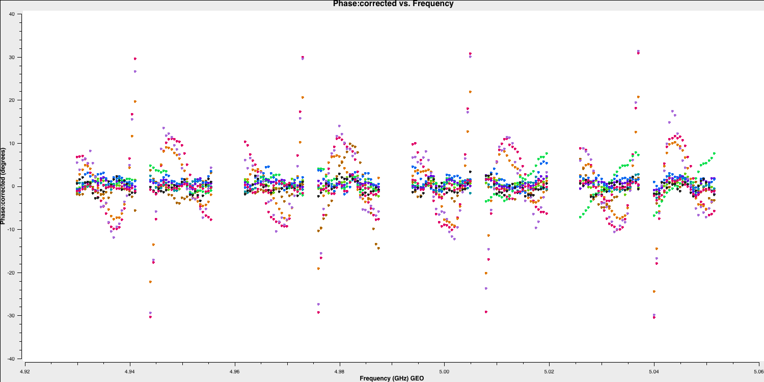
As you can see, the phases are flattened, which is positive. However, if we try a different time range (we have used a time range of 13:18:00~13:20:00 in the plot below), the phases still exhibit slopes across the data, but the jumps between the spectral windows have been removed. The elimination of these jumps allows us to merge the spectral windows, providing us with a much larger signal-to-noise ratio to work with. This is what we will accomplish in the next section.
5B. Multi-band delays
In the next steps, we will combine the spectral windows to solve for multi-band delays and track the changes in the delay signal throughout the observation. This effectively resolves the full phase equation and derives phase, delay, and rate corrections for all antennas relative to a reference antenna.
To do this, we need to use the combine input of the fringefit task to use all spectral windows at once, and we will set the averaging time (or solution interval) to 60 seconds. The choice of solution interval should be determined to ensure adequate S/N for obtaining good solutions while maintaining short enough timescales to track changes in delays, rates, and phases.
Note that because one of our phase calibrators (1848+283) is very bright, we can use it to derive both the instrumental delays and the time-dependent delays. In standard VLBI observations, scans of very bright sources serve as fringe finders for correlation. These scans are also used to derive the instrumental delays (remember that for instrumental delays, we need high S/N in each spectral window, so the source must be very bright!).
After this, we will use the phase calibrator as the time-dependent delay, phase, and rate calibrator. This also considers the phase differences induced by the atmosphere throughout the observation. A key premise of our phase calibrator selection is that these sources should be located close to the target source. This enables us to assume that the solutions derived over time for the phase calibrator are approximately correct for the target field since the signal path through the atmosphere is similar. The instrumental delay calibrator does not need to be near the target field because we are correcting for delays induced by instrumental differences, which are largely independent of the antennas' pointing direction.
- Let's perform the multi-band fringe fitting. Note that we have two phase calibrators (1848+283 and J1640+3946), so to save time, we will conduct the initial fringe fitting on both calibrators.
# In CASA
default(fringefit)
vis='n14c3.ms'
caltable='n14c3.mbd'
field='1848+283,J1640+3946'
solint='60s'
zerorates=False
refant='EF'
combine='spw'
corrdepflags=True
minsnr=30
gaintable=['n14c3.gcal', 'n14c3.tsys','n14c3.sbd']
interp=['nearest','nearest,nearest','nearest']
parang=True
fringefit()
This step may take a while, depending on your computer's specifications, so go get a coffee. The minsnr parameter needs to be set carefully so that we don't pass erroneous solutions. In this experiment, all of the phase calibrators are bright, so a high S/N, such as 30 can be used here. However, many phase calibrators are not this strong, so an S/N threshold of 5 or even 3 may have to be used to converge on enough good solutions.
Finding effective solutions often involves trial and error. However, here are some tips to assess whether your solutions are effective:
- The phases, rates, and delays should vary smoothly if the solutions are effective. If the solutions resemble noise (with large ranges), you may need to increase the averaging interval or the S/N threshold. However, you do not want to raise the S/N too high to the point that solutions cannot converge.
- CASA will inform you of the number of solutions that fail in the logger. By default, CASA will flag the ranges where solutions fail when the calibration tables are applied. This is an easy way to remove all of your good data! Typically, around 5% or fewer failed solutions are acceptable!
Let's apply these tips to the execution of fringefit that we just carried out. First, we will check the logger to see if any solutions failed. You should encounter this somewhat cryptic message:
2025-03-02 09:04:08	INFO	calibrater::solve	Finished solving.
2025-03-02 09:04:09	INFO	fringefit::::casa	Calibration solve statistics per spw:  (expected/attempted/succeeded):
2025-03-02 09:04:09	INFO	fringefit::::casa	  Spw 0: 38/38/38
2025-03-02 09:04:09	INFO	fringefit::::casa	  Spw 1: 0/0/0
2025-03-02 09:04:09	INFO	fringefit::::casa	  Spw 2: 0/0/0
2025-03-02 09:04:09	INFO	fringefit::::casa	  Spw 3: 0/0/0
2025-03-02 09:04:09	INFO	fringefit::::casa	  Spw 4: 0/0/0
2025-03-02 09:04:09	INFO	fringefit::::casa	  Spw 5: 0/0/0
2025-03-02 09:04:09	INFO	fringefit::::casa	  Spw 6: 0/0/0
2025-03-02 09:04:09	INFO	fringefit::::casa	  Spw 7: 0/0/0
2025-03-02 09:04:10	INFO	fringefit::::casa	Task fringefit complete. Start time: 2025-03-02 11:56:23.794540 End time: 2025-03-02 12:04:09.582499
2025-03-02 09:04:10	INFO	fringefit::::casa	##### End Task: fringefit            #####
2025-03-02 09:04:10	INFO	fringefit::::casa	##########################################
You can see that all the solutions are contained in spectral window 0 (spw). This is because we combined the spws, and so CASA puts the solutions into the first spw for bookkeeping. This means we will need to manually specify which spws these solutions are applied to later. You can also see that CASA has attempted 38 solutions and succeeded with all of them! This is the first positive indicator that the solutions are effective.
- Next, we need to ensure the quality of these solutions by inspecting the calibration table. The fringe fitting solves for delays, phases, and rates, so we should check all of these. We will first check the delays.
default(plotms)
vis='n14c3.mbd'    # Name of the calibration file
xaxis='time'       # x-axis
yaxis='delay'      # y-axis
gridrows=2         # number of rows to plot
gridcols=3         # number of columns so total plots = 6 = 2x3
coloraxis='corr'   # colour points by polarisation
iteraxis='antenna' # iterate over the antennae (i.e. each plot is different antenna!)
plotms()
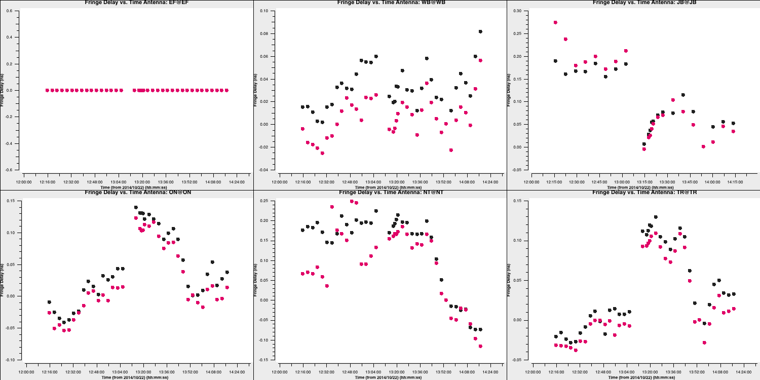
You can see that the delays mostly vary smoothly over time, indicating that the solutions for both phase calibrators are good! Additionally, note that EF is zero because this is the reference antenna, and the delays are measured relative to this antenna.
- Next, we should check the phase solutions. We will simply use the
tgetcommand again, as you only need to change one parameter inplotms:
tget(plotms)
yaxis='phase'
go()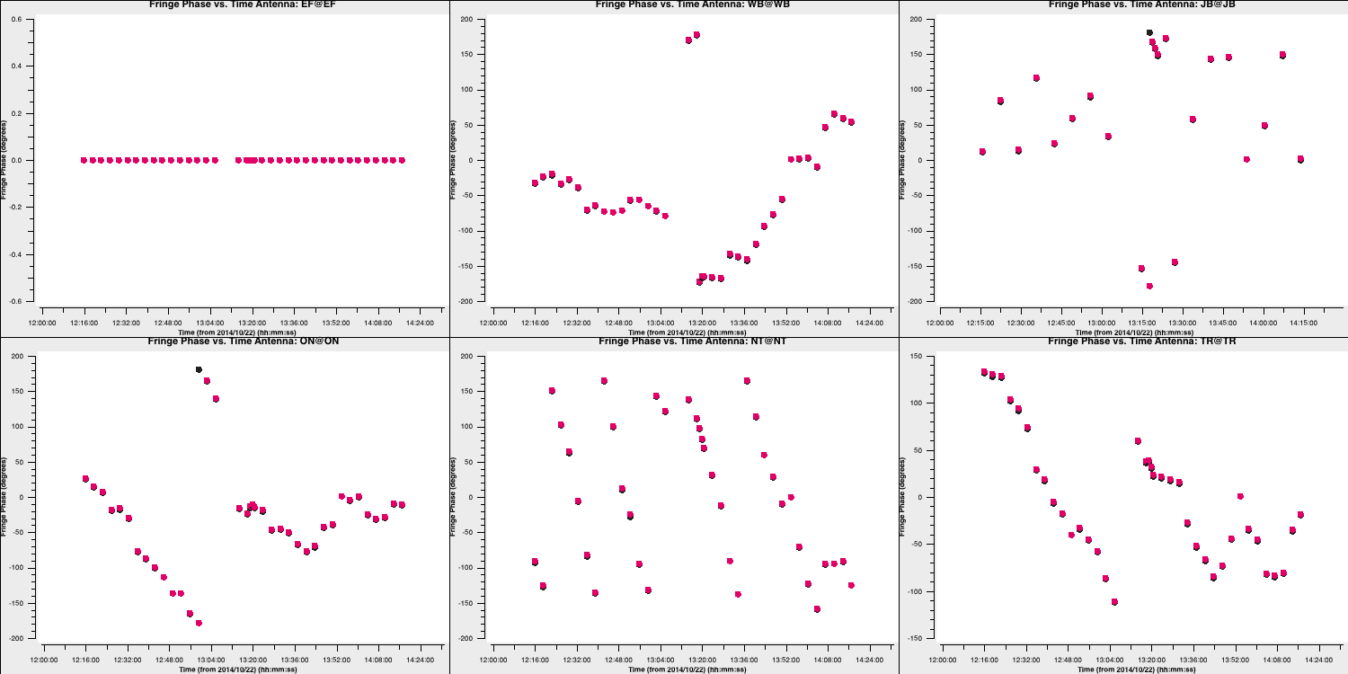
These also change smoothly over time (mostly!), so we can be pleased with them. Finally, let's review the rates (I'll let you determine how to plot this):
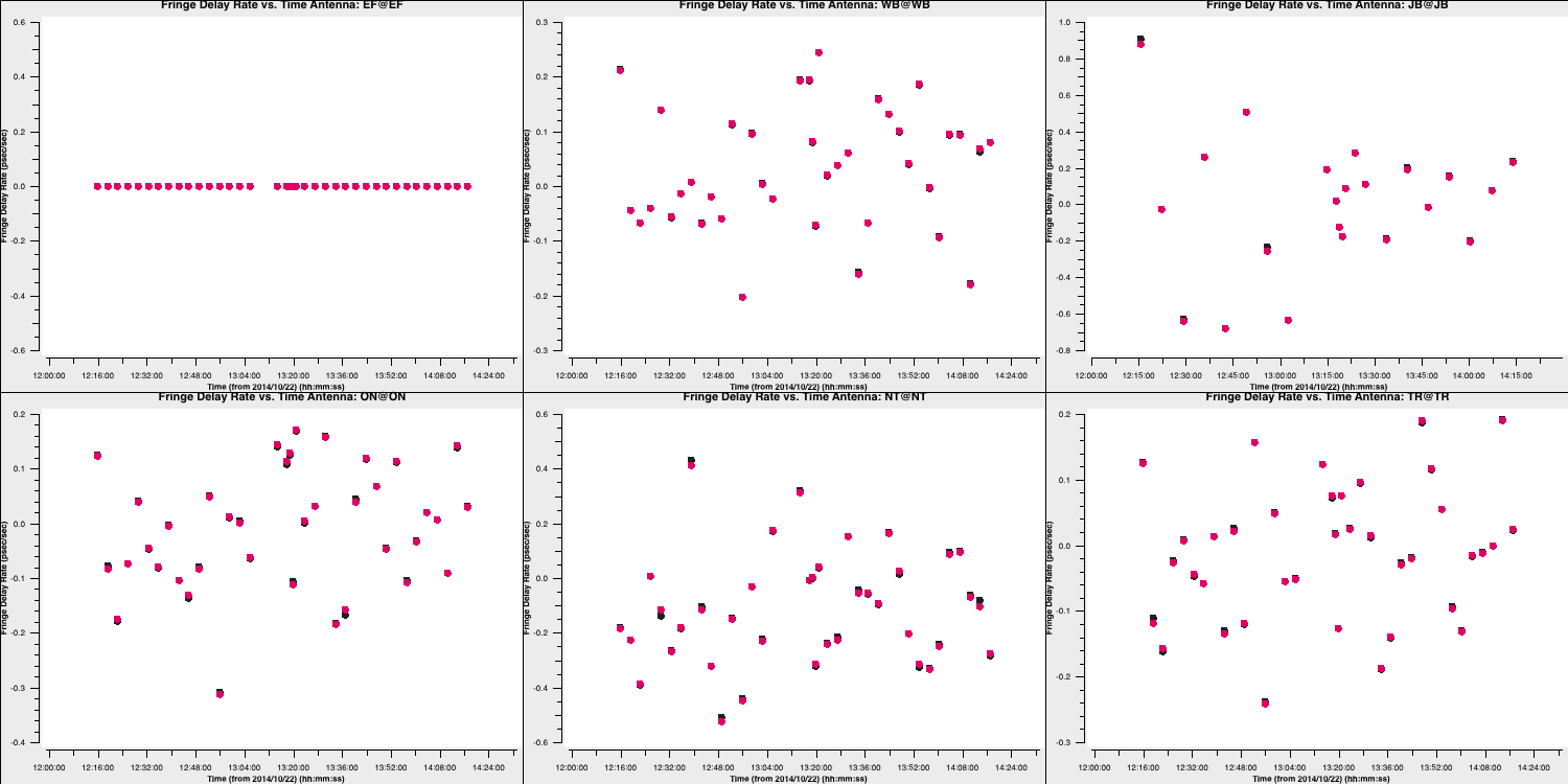
These solutions are somewhat noisier, but note that the scale is significantly smaller. This should also be acceptable. Let's apply these solutions to view the results. Note that since we apply these solutions to our target fields, we need to linearly interpolate the multi-band fringe fitting, as the correct phases, delays, and rates for the target field are expected to be between the two phase calibrator scans surrounding it. Furthermore, we aim to apply the singular solutions from the multi-band delay to all spectral windows; thus, we use the spwmap parameter to map the solutions from spw 0 in the multi-band delay table to the other eight spectral windows (hence the 8*[0]).
- Our
applycalcommand is therefore:
default(applycal)
vis='n14c3.ms'
field='1848+283,J1849+3024'
gaintable=['n14c3.gcal', 'n14c3.tsys', 'n14c3.sbd', 'n14c3.mbd']
interp=['nearest', 'nearest,nearest', 'nearest', 'linear']
spwmap=[[], [], [], [0,0,0,0,0,0,0,0]]
parang=True
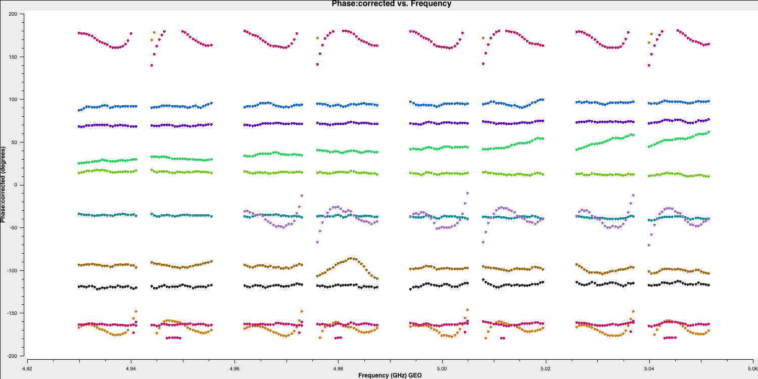
applycal()Let's examine our phases on each baseline as a function of frequency based on the original scan used to calculate the instrumental delay:
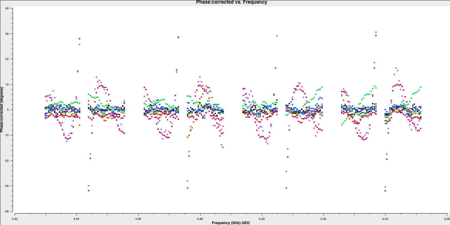
And for the other scan, where the baseline phases had only the instrumental delay applied:
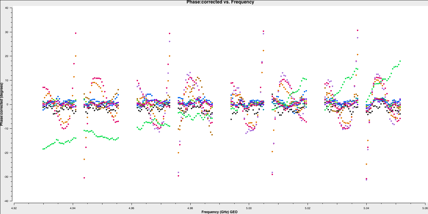
You can see that most of the phases have now lined up, and the slopes we observed earlier have mostly disappeared. We will refine this calibration in Part 2.
6. Bandpass calibration
As you may have noticed before, when we flagged the edge channels, the amplitude versus frequency of your data has a distinctive shape. This is due to the differing sensitivity of the telescope receiver systems at varying frequencies. Let's take another look at this in plotms:
default(plotms)
vis='n14c3.ms'
xaxis='frequency'
yaxis='amplitude'
ydatacolumn='corrected'
antenna='EF'
correlation='LL,RR'
coloraxis='baseline'
timerange='13:53:20.0~13:54:20.0'
avgtime='60'
plotms()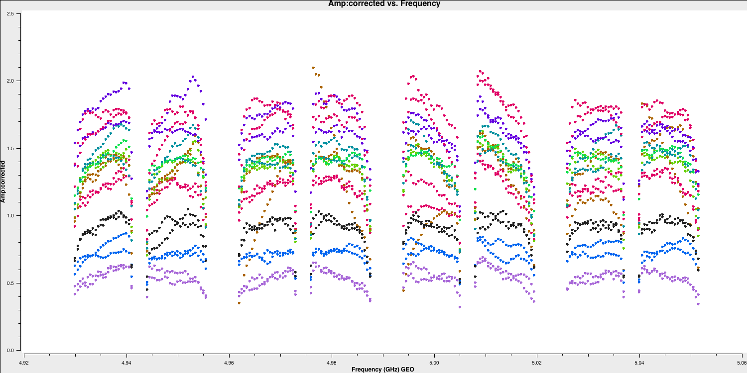
We can use the task bandpass to correct this, as it calculates a complex gain (amplitude and phase) that addresses the sensitivity differences across the bandwidth. With phases, rates, and delays all removed, this is the only calibration issue remaining (mostly!). Again, this is an instrumental effect, so we would not expect it to change over time.
We can use our instrumental delay calibrator again for this. From instrumental delay calibration, we know there is sufficient S/N per spw. However, to follow the exact shape of the bandpass, we now need to ensure we have enough S/N per channel! We can achieve this by combining all of the scans together (valid as the bandpass response shouldn't change over time).
- Input the following to derive the bandpass corrections:
default(bandpass)
vis='n14c3.ms'
caltable='n14c3.bpass'
field='1848+283'
gaintable=['n14c3.gcal', 'n14c3.tsys', 'n14c3.sbd', 'n14c3.mbd']
interp=['nearest','nearest,nearest','nearest','linear']
solnorm=True
solint='inf'
corrdepflags=True
refant='EF'
bandtype='B'
spwmap=[[],[],[], 8*[0]]
parang=True

bandpass()
The bandpass correction should follow the shape of the amplitude response we examined earlier. Note that we set the solnorm parameter, which means the calibration solutions are normalised to unity, thus preserving the total amplitudes of the data. In this case, we want to do this because our flux density scaling is done a priori, and this needs to be preserved.
- Let's plot the bandpass corrections, starting with the amplitude corrections (it's up to you to figure out the commands yourself this time!):
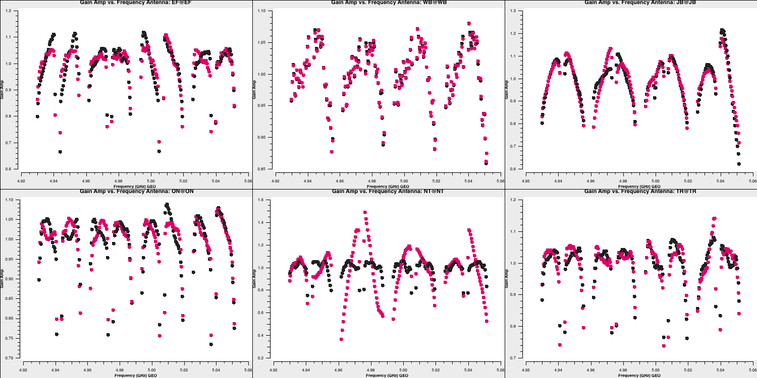
Note that, when CASA calibration tables are applied, the solution tables are divided by the visibilities, which contrasts with the old software, AIPS, where solutions are multiplied by the visibilities. This means that the amplitude solutions shown here should roughly correspond to the visibilities as illustrated earlier. Let's plot the phases as well. These should follow the wiggles we observed within each spectral window.
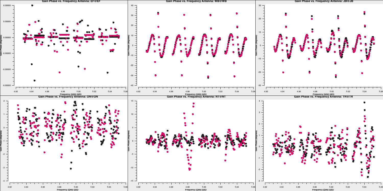
The Effelsberg telescope serves as our reference antenna, but the phases appear noisy. However, if you examine the y-axis scale, you will notice that these variations are on the order of $10^{-7}\,\mathrm{deg}$. These are primarily computational floating-point errors that hold no significant impact!
- These solutions look good, so we should apply this table to the data using
applycal:
default(applycal)
vis='n14c3.ms'
field=''
gaintable=['n14c3.gcal', 'n14c3.tsys', 'n14c3.sbd', 'n14c3.mbd','n14c3.bpass']
interp=['nearest','nearest,nearest','nearest','linear','nearest,nearest']
spwmap=[[], [], [], 8*[0],[]]
parang=True

applycal()
- Let's have a look at what this has done to the visibilities of 1848+283. Firstly the amplitudes:
default(plotms)
vis='n14c3.ms'
xaxis='frequency'
yaxis='amplitude'
ydatacolumn='corrected'
antenna='EF'
correlation='LL'
coloraxis='baseline'
field='1848+283'
plotms()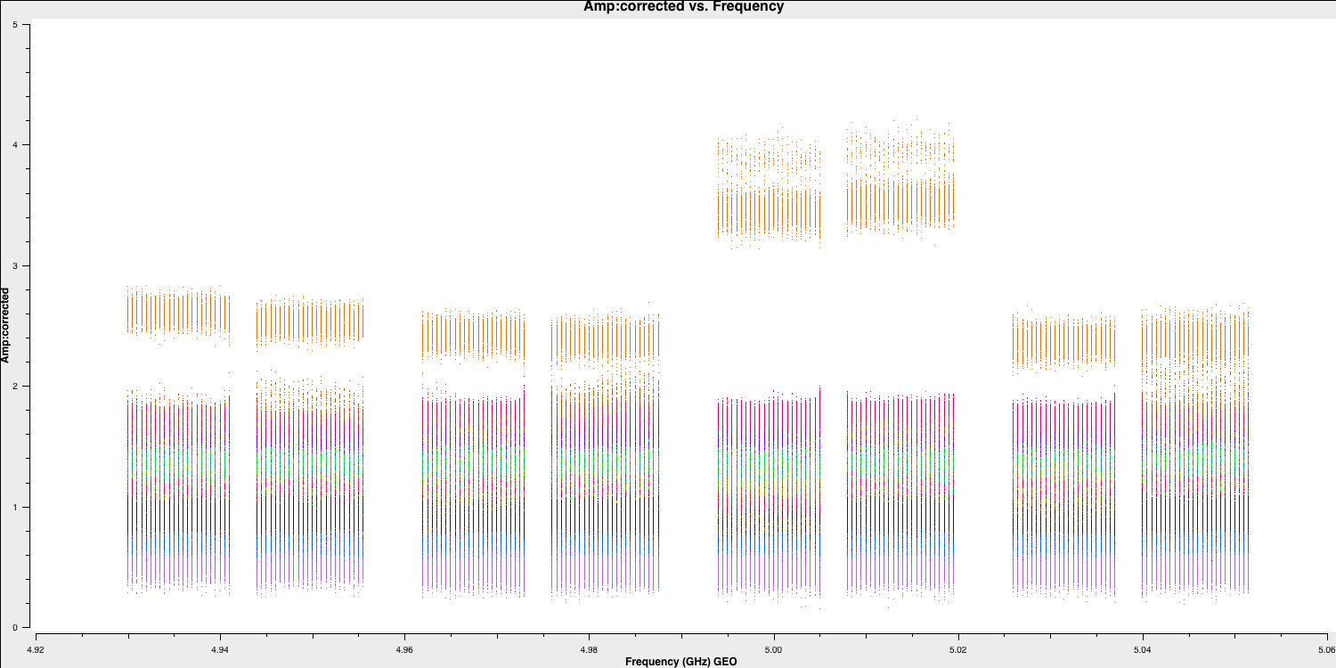
We can see that the amplitudes are scaled correctly and the bandpass shape has disappeared. The plot is coloured by baseline, and the differences in amplitudes are either due to amplitude errors or varying flux across different baselines and spatial scales because of the structure of the phase calibrator. If this is a true point source, we would expect the flux on all baselines to be the same. We will correct these amplitudes later using self-calibration. Now, let's examine the phases as well:
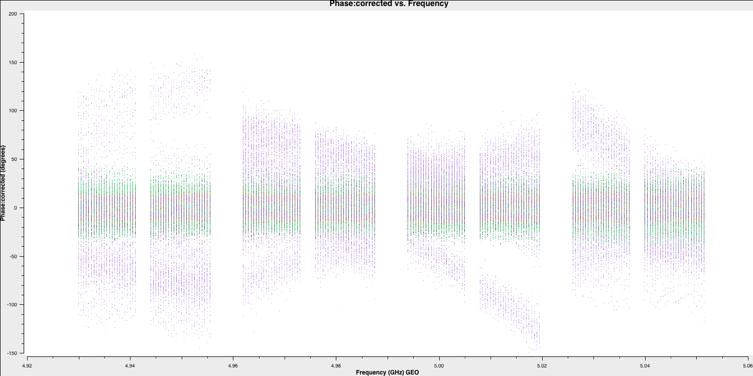
Here, the phases are mostly near zero, except for one antenna (SH), which appears to be erroneous. We will try to address this a little later. For now, this is acceptable, and we can proceed to separate this data into the two phase-reference target pairs for Parts 2 and 3!
7. Split out phase-ref - target pairs
The final task we need to complete is splitting the pairs of target and phase reference sources. This not only prepares us for parts 2 and 3 of this workshop but also ensures we have backup copies in case future data is corrupted or deleted. We use the task split to accomplish this, and it is straightforward to use:
## In CASA
default(split)
vis='n14c3.ms'
outputvis='J1640+3946_3C345.ms'
field='J1640+3946,3C345'
datacolumn='corrected'
split()
## In CASA
default(split)
vis='n14c3.ms'
outputvis='1848+283_J1849+3024.ms'
field='1848+283,J1849+3024'
datacolumn='corrected'
split()This completes Part 1 of the tutorial. You should have been introduced to amplitude calibration, data inspection, and flagging, fringe fitting, and bandpass calibration. In the following two parts, we will further investigate phase referencing, along with imaging and the self-calibration technique. If you have any further questions, ask the DARA trainer or continue to Part 2.
Part 2: Calibration & imaging of J1849+3024