
Spectral Line Workshop
NGC660 Hydrogen Absorption
In the second of the DARA data reduction tutorials, we will reduce a spectral line dataset collected with the European VLBI Network. The aim of this tutorial is to introduce the various additional calibration and imaging steps associated with spectral line data. Additionally, we will focus on extracting some science from the results, a topic that was missing from the first tutorial. You should use CASA version 6.5.4 on Linux and version 6.6.5 on Mac OS. Installation instructions are available on the EVN continuum tutorial homepage. If you wish to use CASA version 6.3 or higher for this tutorial, please follow this link, or access the CASA version 5 tutorial through this link.
This workshop was originally curated by Anita Richards and has been subsequently updated by Jack Radcliffe.Please use the contact form at the bottom of the page if you encounter any issues or have general questions about this workshop. If you are satisfied, please follow the instructions below!
Data download instructions
Before we start, we need to ensure that all the necessary data and scripts are present. Note that this tutorial should only take up around 7-10 GB on your hard drive. These files should already be on your filesystem (ask the trainers!). If you are working remotely, use the following buttons to download these data. If your internet is slow, download the smaller tar ball, i.e., NGC660 data (624MB). The included files are those with the *, and the other data files can be generated from these. If your internet is fast, download the complete tar ball, i.e., NGC660 data all (1.2GB):
Extract the tar file and you should find the following files in your directory:
*NGC660.FITS*- UVFITS data set with instrumental and calibration source corrections applied - needed to run from the beginning of this script.NGC660shift.ms.tar.gz- data set for beginning at step 8 (create this yourself if progressing through steps 1-7).NGC660line.image.tar.gzandNGC660contap1.image.tar.gz- images for analysis (you will create these yourself, but just in case...).*NGC660.py*- script outlining the steps on this web page.*NGC660.flagcmd.txt*- flags for step 2.
In this tutorial, we will reduce some spectral line data of the starburst galaxy NGC660. You will notice that many of the steps are similar to those before; however, there are some extra complications. Before we start, please follow the instructions to download the relevant datasets and scripts, and then we can begin. The guide starts with a dataset that has already been flagged and calibrated using the instrumental corrections and calibration derived from astrophysical sources, including phase referencing. This was done in AIPS, and the split-out, calibrated data NGC660.FITS is in UVFITS format.
Table of Contents
- Background on NGC660
- Improving the calibration of NGC660
- Convert data to MS and get information (step 1)
- Plot visibility spectrum, identify continuum, flag bad data (step 2)
- Plot amplitude against uv distance (step 3)
- Make the first continuum image (step 4)
- Find the source position (step 5)
- Phase shift the data and make an image (step 6-7)
- Self-calibrate (step 8)
- Image the calibrated continuum, subtract continuum from the line and make the line cube
- Image cube analysis
1. Background on NGC660
NGC 660 is an unusual starburst galaxy featuring a polar ring, located approximately 13.5 Mpc away. This peculiar configuration likely results from a major merger event between two galaxies around one billion years ago or the capture of matter from a nearby galaxy that subsequently formed the ring structure.
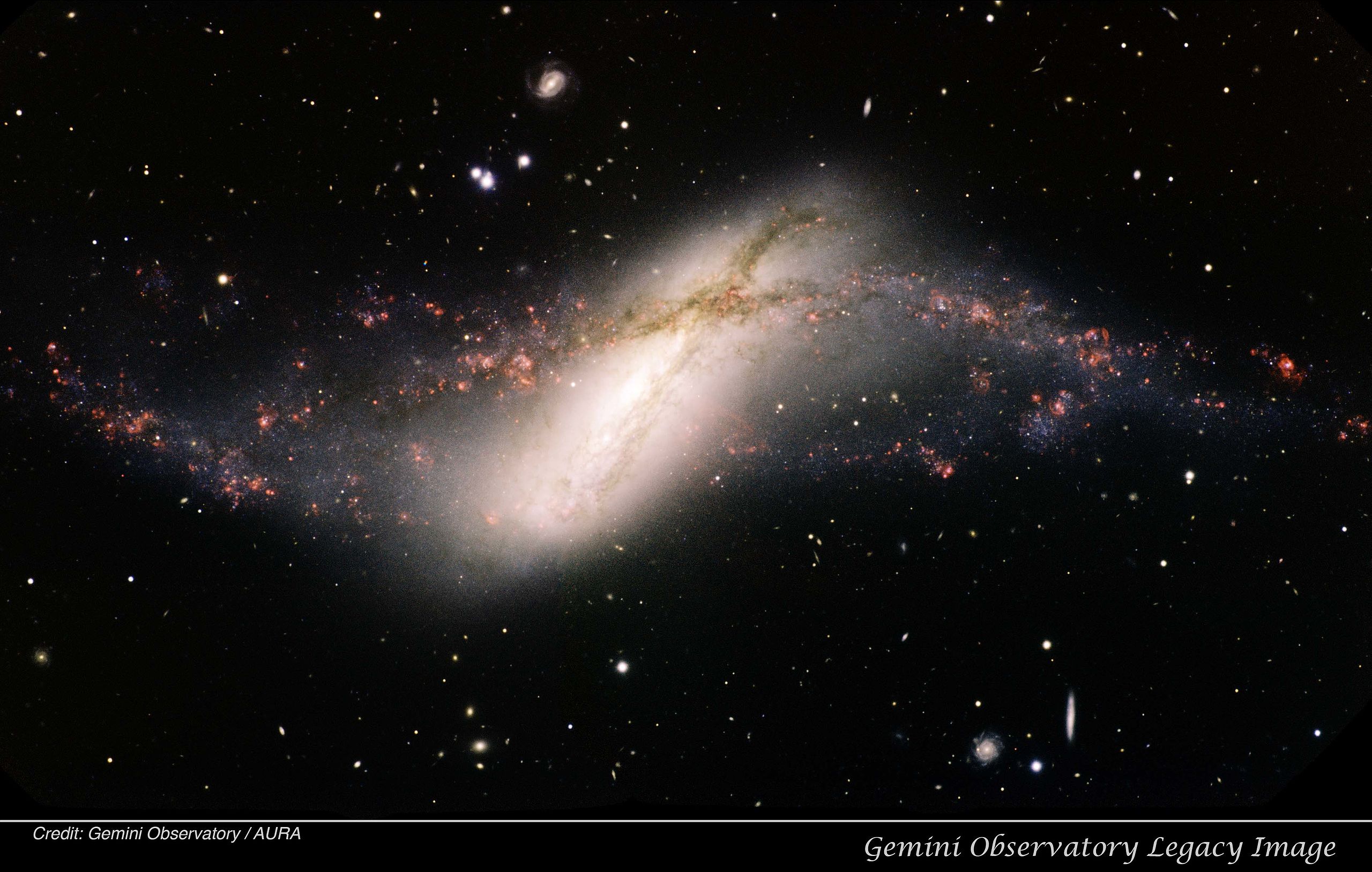
The central area contains a region of intense star formation. Radio observations initially suggested that the centre of the galaxy might harbour a supercluster of stars; however, between 2008 and 2012, this understanding shifted dramatically. Observations detected an outburst that was approximately ten times brighter than a supernova explosion. A new continuum radio source emerged, accompanied by absorption lines that indicated this source originated from the accretion of matter onto the central black hole. The observations conducted using the European VLBI Network aimed to determine and confirm the Active Galactic Nuclei origin of this source and explore any inflows or outflows of neutral gas through HI absorption lines. This is the data we will be analysing in this tutorial. To read more about the results of these observations, see Argo et al. 2015.
2. Improving the calibration of NGC660
To use this guide, you can either run the script (NGC660.py) step by step, copy and paste each task from this web page, or enter parameters line by line (in which case you should omit the comma at the end of each line). If you are working from this web page, you need to input some values yourself, but these are already included in the script. Please ensure that you try to understand what each step does; otherwise, you will learn nothing!
The guide begins with a dataset that has already been flagged and calibrated using instrumental corrections and calibrations derived from astrophysical sources, including phase referencing.
A. Convert data to MS and get information (step 1)
These data come from AIPS, which exports visibilities in UVFITS format. Therefore, we need to convert them from UVFITS to a measurement set using the CASA task importuvfits.
os.system('rm -rf NGC660.ms*')
importuvfits(fitsfile='NGC660.FITS',
				 vis='NGC660.ms')
AAs usual, one of the principles of effective data reduction is comprehending the data. Let's use listobs to examine the contents of the data.
os.system('rm -rf NGC660.ms.listobs')
listobs(vis='NGC660.ms',
		listfile='NGC660.ms.listobs')
Examine the listobs output to understand what data is present. You should observe that there is only one source and one spectral window (spw) with 1024 channels. In total, 7 antennas are available.
B. Plot visibility spectrum, identify continuum, flag bad data (step 2)
To begin, we need to identify where the continuum emission and spectral line features are within the band. This ensures that we can successfully subtract the continuum emission from the spectral line absorption/emission and also confirms that we do not confuse the spectral line with RFI, preventing it from being flagged during the process. In most projects involving spectral line data, the project proposal will include the spectral lines we are searching for, allowing you to extract this information. However, in the absence of such information, there are two ways to determine the location of the spectral lines.
If the spectral line is strong enough (as is the case with this data), we can plot the data (and average it over time) to observe the lines. However, for weak lines, we must use the source's distance to estimate the location of the lines in frequency space. We will do this for this data set for completeness. NGC660 is approximately 13.5 Mpc away, which corresponds to a redshift of 0.003. We are searching for HI absorption, whose rest frame frequency is 1420.405751 MHz; therefore, our observed line frequency should be close to $1.420405751/1+z = 1.4160961\,\mathrm{GHz}$. Note that the rest frame frequencies of spectral lines can be found using the Splatalogue database or the slsearch CASA task.
plotms for visualisation. As previously mentioned, EF (Effelsberg) is the most sensitive antenna and serves as the reference antenna. We will plot amplitude against channel. The end channels and some near channel 775 have already been flagged. The absorption is clearly visible and consists of two components.
## In CASA
plotms(vis='NGC660.ms',
	   xaxis='channel',
	   yaxis='amp',
	   avgtime='36000',
	   antenna='EF&*',
	   iteraxis='baseline',
	   avgscan=True)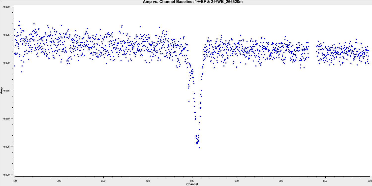
Select the continuum channel ranges. As you can see, the spectral line deviates from the expected frequency of $1.416\,\mathrm{GHz}$ calculated earlier and displays two components. This occurs because the absorption regions possess their own intrinsic velocity towards and away from us along the line of sight. This broadens the area we intend to classify as a spectral line within the spw. Therefore, we aim to exclude the 100 channels surrounding the line and define this as the continuum emission region using the variable contchans (fill in xxx and yyy). Enter this into CASA:
contchans='0:100~xxx;yyy~900'To ensure we obtain the best images of our line, we should check for any additional bad data. Remember that flagging is an iterative process, and some low-level bad data will only become apparent after you partially calibrate the data. In this data, initial flagging was performed before phase referencing, but the calibration of the target has revealed more bad data.
Let's plot the data to identify the bad data, and we will use Mark and Locate to determine the baselines or antennas involved. Please note that we do not want to flag the high data, as these are mostly just mis-scaled and will be calibrated later.
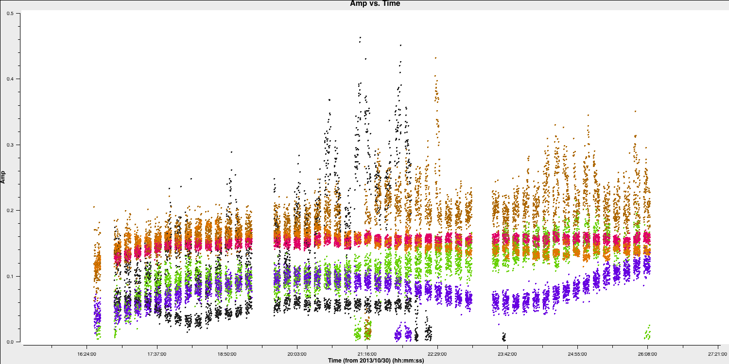
The bad data here consists of the scans where the visibilities drop to zero amplitude. These occur across various scans, primarily on the Onsala (ON) and Medicina (MC) telescopes, and are mainly confined to single polarisations. Normally, when flagging data, you would want to create a flag file to record this, which enables you to precisely replicate the flagging if you need to recalibrate these data.
To save time, we have provided the pre-made flag file. Use your favourite text editor to open NGC660.flagcmd.txt. This file contains the commands to flag the data and allows you to compare this with the information you received by using the Mark and Locate function of the plotms task.
If you are satisfied that these conform, we can use the flag file to mark this bad data. We will use flagmanager to create a backup of the current flags (in case we need to revert) and then use flagdata to apply the flag file:
flagmanager(vis='NGC660.ms',
			mode='save',
			versionname='prelist')

flagdata(vis='NGC660.ms',
		 mode='list',
		 inpfile='NGC660.flagcmd.txt')
With this in place, we should reload plotms to ensure that all the bad data is removed (use the tget command!)
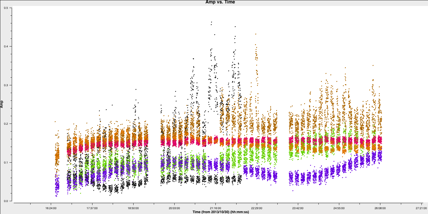
Hooray, all of the bad data is gone!
C. Plot amplitude versus uv (step 3)
Since we have excised the bad data and the phase referencing has already been completed, we should prepare for our first imaging run to perform self-calibration on this dataset. First, we need to determine the imaging parameters. The most crucial aspect is to identify the cell parameter, which can be derived from the amp vs. uv plot:
plotms(vis='NGC660.ms',
	   xaxis='uvwave',
	   yaxis='amp',
	   avgchannel='801',
	   avgtime='30',
	   coloraxis='antenna1',
	   overwrite=True)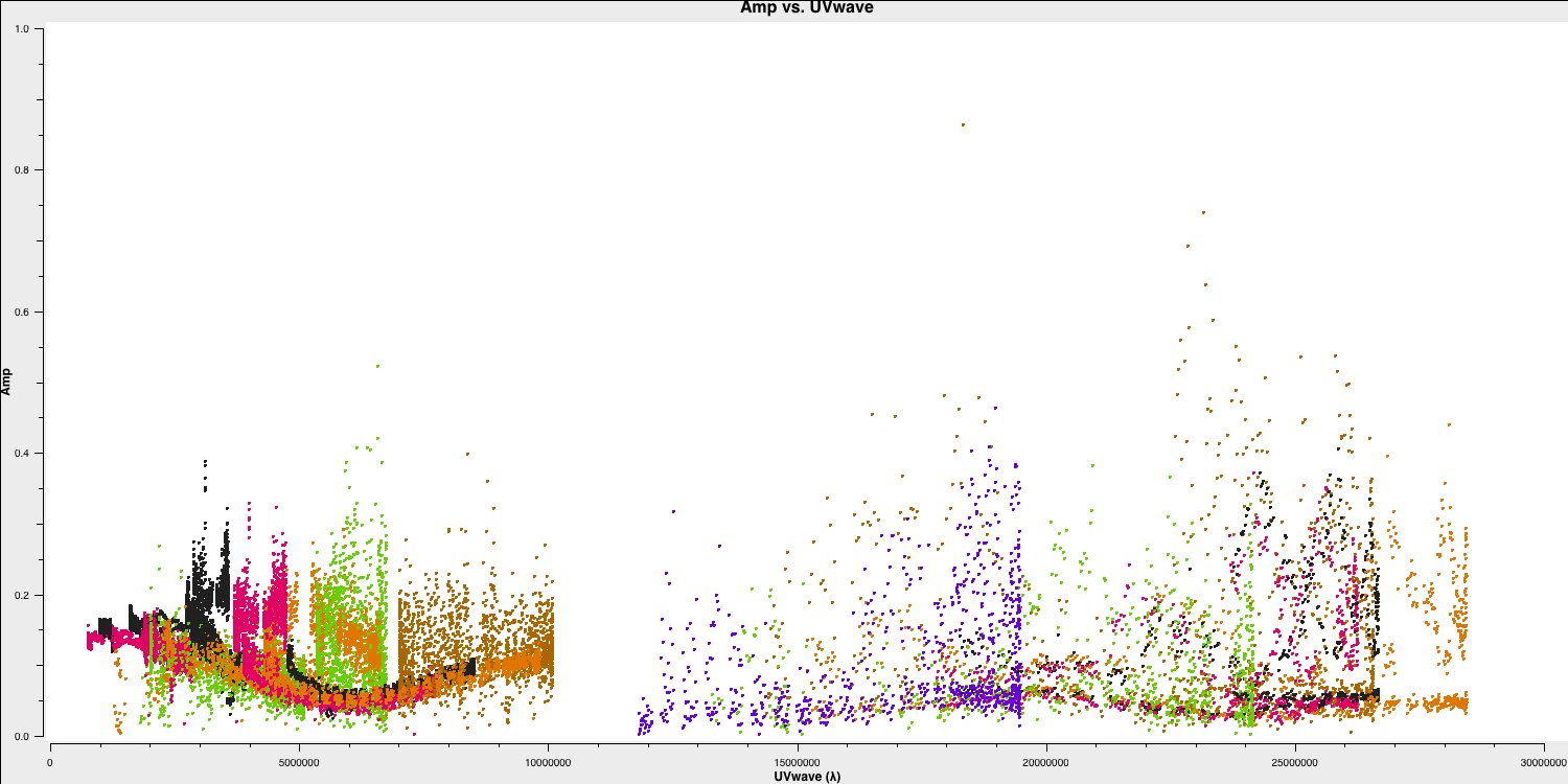
Remember from part 2 of the EVN continuum tutorial that we used this plot to estimate the effective resolution of our interferometer, given that the resolution of an interferometer is expressed as $ abla/ext {B}$, where ext {B} represents the maximum baseline length. Based on this, we derived the following equation to determine the cell size, including the Nyquist sampling parameter $ N_\mathrm{s}$, enabling us to fit to the PSF.
$$\mathrm{cell} \approx \frac{180}{\pi N_{\mathrm{s}}} \times \frac{1}{D_{\max }[\lambda]}[\mathrm{deg}]$$
After working this out, set the cellsize variable in CASA or in the script (it should be between 1.5 and 2.5 milliarcseconds depending on your choice of $N_\mathrm{s}$):
cellsize='xxxmas'D. Make the first continuum image (step 4)
As with many projects, we do not know exactly where the target source is. In this case, the target position was only known to around an astrometric accuracy of around one arcsecond. We therefore want to make a larger image to obtain the target location. We shall use an image size of 1280 (an optimal number for the underlying algorithms i.e. $2^n \times 10$). In addition, we want to avoid the spectral line at the moment so we use the contchans parameter to define the spectral windows.
os.system('rm -rf NGC660cont0.*')
tclean(vis='NGC660.ms',
		imagename='NGC660cont0',
		field='NGC660',
		specmode='mfs',
		threshold=0,
		spw=contchans,
		deconvolver='clark',
		imsize=[1280,1280],
		cell=cellsize,
		weighting='natural',
		niter=100,
		interactive=True,
cycleniter=25)from casagui.apps import run_iclean
os.system('rm -rf NGC660cont0.*')
run_iclean(vis='NGC660.ms',
imagename='NGC660cont0',
field='NGC660',
specmode='mfs',
threshold=0,
spw=contchans,
deconvolver='clark',
imsize=[1280,1280],
cell=cellsize,
weighting='natural',
niter=100,
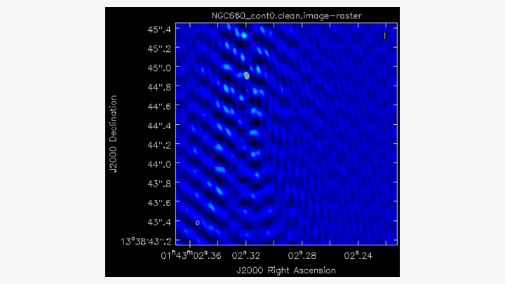
cycleniter=25)You should notice that the source is offset from the pointing centre, and we will adjust this soon. Clean the dirty image to produce a clear image that should resemble the following.
E. Find the source position (step 5)
Open the image in the viewer(Linux) or CARTA (MacOS) to obtain the same image as above. We want to adjust our visibilities so that the peak of the emission is at the centre of the image. This adjustment simplifies removing the continuum emission from the spectral line. CASA performs a phase shift to adjust the phase centre of the observation. However, we first need to determine the location of the peak brightness.
We can do this in two ways: we can draw a region around the source and interactively fit a 2-D Gaussian component using the Region Fit tab, as shown below.
One important aspect of this method is that we obtain our position from the logger rather than the viewer panel (in the case of the viewer - Linux). This is because the accuracy of the returned position in the viewer panel is not sufficient.
The second method involves using the task imfit to perform the same fitting, which is recommended for MacOS users. The advantage of this approach is that we can place it in a script for automatic execution, should this step need to be repeated. To use the imfit task, we must define a box around the source where fitting will occur. This is inputted into imfit as box='blc x, blc y, trc x, trc y', where trc denotes the top right corner and blc indicates the bottom left corner.
Use the viewer/CARTA to identify these positions and set the variable boxsize accordingly. Next, let's run imfit using the following code:
imfit(imagename='NGC660_cont0.image',
	  box=boxsize,
	  logfile='NGC660_contpeakpos.txt')
Using either of these methods, you should recover a peak brightness position of the source to be near $\mathrm{RA} \approx 01^\mathrm{h}43^\mathrm{m}02.319403^\mathrm{s}$ and $\mathrm{Dec} \approx +13^{\circ}38^\mathrm{m}44.905554^\mathrm{s}$. In the next step, we will shift our data set to this position.
F. Phase shift the data and make an image (step 6-7)
The task phaseshift is used to calculate and apply the phase shifts needed to position the source at the centre of the field, enhancing the accuracy of continuum subtraction and making imaging more convenient. We need to apply the position derived earlier and set the phasecenter parameter.
phaseshift(vis='NGC660.ms',
	   outputvis='NGC660shift.ms',
	   phasecenter='J2000 HHhMMmSS.SSSSSS +DDdMMmSS.SSSSSS')
This task creates a new measurement set called NGC660shift.ms, which places the source at the centre of the field. We will use this measurement set from now on and should proceed with imaging it:
os.system('rm -rf NGC660cont1.*')
tclean(vis='NGC660shift.ms',
	   imagename='NGC660cont1',
	   field='NGC660',
	   specmode='mfs',
	   threshold=0,
	   spw=contchans,
	   deconvolver='clark',
	   imsize=[320,320],
	   cell=cellsize,
	   weighting='natural',
	   niter=50,
	   interactive=True,
cycleniter=25)os.system('rm -rf NGC660cont1.*')
run_iclean(vis='NGC660shift.ms',
imagename='NGC660cont1',
field='NGC660',
specmode='mfs',
threshold=0,
spw=contchans,
deconvolver='clark',
imsize=[320,320],
cell=cellsize,
weighting='natural',
niter=50,
cycleniter=25)
Clean this image, and you should see that the source is now centred. Note that we can use a smaller image size since we have found the source and can see that it is compact. This reduces computing time when imaging. Finally, we need to generate the $\texttt{MODEL}data column, so we use the ft task:
ft(vis='NGC660shift.ms',
   field='NGC660',
   model='NGC660cont1.model',
   usescratch=True)
We are now ready to perform self-calibration; however, we first want to track the improvement in image fidelity achieved with each calibration step. The simplest approach is to monitor the signal to noise ratio (S/N), which improves with better calibration. We can automate this using the imstat task. We need to define two boxes: one off-source to measure the rms noise and one on-source to measure the peak brightness. Remember, you can use imview/CARTA for this. The ratio of these will give us the S/N ratio.
rms=imstat(imagename='NGC660cont1.image',
		   box='offblcx,offblcy,offtrcx,offtrcy')['rms'][0] # Set blc and trc of a largest box well clear of the source
peak=imstat(imagename='NGC660cont1.image',
			box='blcx,blcy,trcx,trcy')['max'][0] # Set blc and trc to enclose the source
print('Peak %6.3f mJy/beam, rms %6.3f mJy/beam, S/N %6.0f' % (peak*1e3, rms*1e3, peak/rms))
Please note that the notation for the box is the same as what we used for imfit.
You should obtain a peak brightness of $S_\mathrm{p} \approx 0.116\,\mathrm{Jy\,beam^{-1}}$, rms noise of $\sigma \approx 0.009\,\mathrm{Jy\,beam^{-1}}$ and so a $\mathrm{S/N}\approx 12$.
G. Self-calibrate (step 8)
The visibility amplitudes indicate good signal-to-noise across all baselines to EF. The data are mostly well-calibrated, but there are some discrepant amplitudes noted above, so we should solve for amplitude and phase. Note that the parallactic angle correction was applied before creating the data set we loaded. Referring to the zoomed plot of amplitude versus time at the end of Step 2, the systematic trends in the amplitude errors appear to exceed the noise scatter on timescales of 20 to 60 seconds, so select a solution interval within this range. We must set solnorm=True as we have already performed flux scaling in the pre-processing steps prior to this workshop.
gaincal(vis='NGC660shift.ms',
		caltable='NGC660.ap1',
		solint='XXXs',
		minsnr=1,
		minblperant=2,
		solnorm=True)

plotms(vis='NGC660.ap1',
	   xaxis='time',
	   yaxis='amp',
	   iteraxis='antenna',
	   coloraxis='corr',
       gridcols=3,
       gridrows=2,
	   plotfile='NGC660.ap1.png')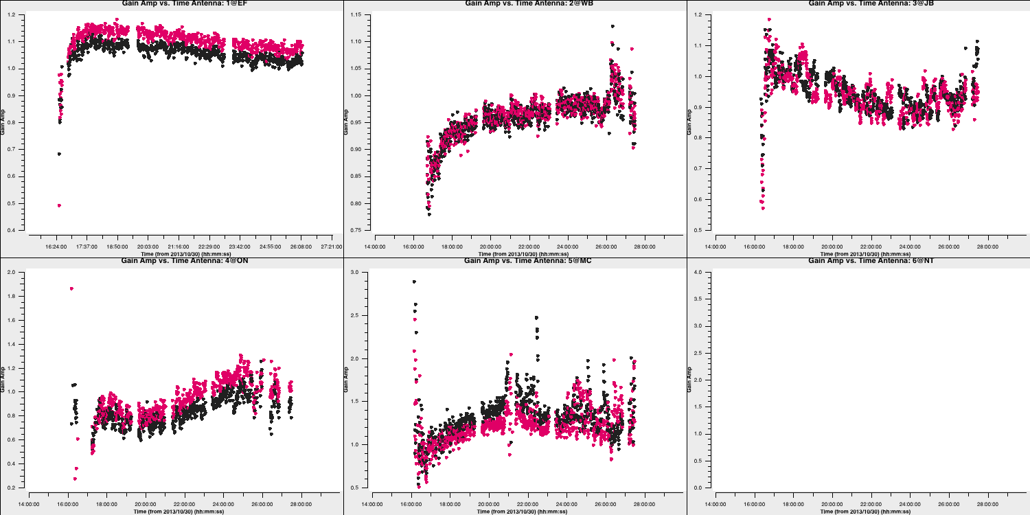
As you can see, these solutions are clean and vary smoothly, so they must be acceptable. If you traverse through the solutions, you'll see that the high amplitudes we observed earlier will be corrected by this table.
Let's apply these to the data.
applycal(vis='NGC660shift.ms',
		 gaintable='NGC660.ap1',
		 applymode='calonly')
3. Image the calibrated continuum, subtract continuum from the line and make the line cube
A. Image the calibrated continuum (step 9)
Important: If you have completed steps 1-7, you should have the file NGC660shift.ms. If not, please move or delete any existing NGC660shift.ms file and unpack a pre-made version using tar -zxvf NGC660shift.ms.tgz.
We want to image the continuum only; therefore, we should use the contchans parameter that we defined earlier to avoid the spectral line. In addition, we derived the cellsize in step 3, so this should also be set. In this tclean iteration, we are going to change the weighting to Briggs's weighting with a robust value of 0. This gives us better resolution, allowing us to distinguish between the core and the jet. Take a look at the imaging lectures to learn more about different weighting schemes.
os.system('rm -rf NGC660contap1.*')
tclean(vis='NGC660shift.ms',
	   imagename='NGC660contap1',
	   field='NGC660',
	   spw=contchans,
	   specmode='mfs',
	   threshold=0,
	   deconvolver='clark',
	   imsize=[320,320],
	   weighting='briggs',
	   robust=0,
	   cell=cellsize,
	   niter=200,
	   interactive=True,
cycleniter=50)os.system('rm -rf NGC660contap1.*')
run_iclean(vis='NGC660shift.ms',
imagename='NGC660contap1',
field='NGC660',
spw=contchans,
specmode='mfs',
threshold=0,
deconvolver='clark',
imsize=[320,320],
weighting='briggs',
robust=0,
cell=cellsize,
niter=200,
cycleniter=50)If we use the same boxes as before, we can see that we now have: $S_\mathrm{p} \approx 0.1283\,\mathrm{Jy\,beam^{-1}}$, rms noise, $\sigma \approx 0.6\,\mathrm{mJy\,beam^{-1}}$ and so a $\mathrm{S/N}\approx 229$. This is a great improvement upon what we had before.
Inspect the image in the viewer/CARTA and double-check this yourself to determine your S/N. You should also observe the core-jet structure appearing with the different weighting scheme we used. The plot below illustrates the structural differences obtained with natural and Briggs (robust=0) weighting applied to the same data. Note that the peak brightness is lower due to increased resolution and a smaller synthesised beam.
B. Subtract the continuum and image the line cube (step 10-11)
The next step is to remove the continuum emission from the spectral line absorption/emission. To do this, we use a task called uvcontsub. This task takes the model of the Fourier Transformed data in the measurement set and subtracts it from the corrected visibility data. First, we need to put our most recent model into the data set:
ft(vis='NGC660shift.ms',
	   model='NGC660_contap1.clean.model',
	   usescratch=True)
Next, we remove this model from the visibilities. We select only the continuum channels and perform linear interpolation (thus, fitorder=1) over the gap where the spectral line exists. The continuum subtraction is computed for each integration.
os.system('rm -rf NGC660shift.contsub.ms*')
uvcontsub(vis='NGC660shift.ms',
		  outputvis="NGC660shift.contsub.ms",
		  fitspec=contchans,
		  fitorder=1)
This generates a new measurement set named NGC660shift.contsub.ms, which should only contain noise in the continuum-only channels.
Now we want to move on to creating our first image cube, which allows us to determine which components are moving towards and away from us. To obtain the correct velocities, we need to set the line rest frequency. We did this earlier when we estimated the location of the line using slsearch, but let's do it again to ensure you understand. Assuming that you only remember the rough rest frequency of the HI 21-cm line, you can obtain an accurate value using the following command:
slsearch(freqrange=[1.408376,1.424376],
		 rrlinclude=False,
		 logfile='NGC660_HIrest.log',
		 verbose=True,
		 append=False)
You should have several lines in the output file NGC660_HIrest.log. Look for atomic hydrogen. The output should resemble the following:
SPECIES       RECOMMENDED        CHEMICAL_NAME   FREQUENCY     QUANTUM_NUMBERS  INTENSITY      SMU2      LOGA        EL        EU  LINELIST
...
t-HCOOH                 * Formic Acid             1.418660 43(7,36)-43(7,37)     -9.89870   4.27423   1179.34717  CDMS
H-atom                  * Atomic Hydrogen         1.420410 2S1/2,F=1-0           -9.06120   0.00026 -14.54125   0.00000   0.06817  JPL
g-CH3CH2OH              * gauche-Ethanol          1.420760 35(7,28)-35(7,29),vt  -9.81460   4.41121 -11.68321 641.53949 641.60767  JPL
...
You should find that HI has a rest frequency of $1.420410\,\mathrm{GHz}$.
Select the line channels between the continuum channels for imaging. The default setting in tclean/run_iclean, which we have used so far, averages all channels to create a continuum map. Now, use specmode='cube' to image each channel separately (or as determined by the parameter width, if you prefer to average for greater sensitivity). Choose the start channel as the end of the first chunk of continuum, and set nchans to the number of central channels that you did not use for continuum (i.e., the number of channels for the output cube, not the original channel number). By default, CASA uses the radio convention for converting the fractional frequency shift to velocity ($v$), that is,
$$v = c \times \frac{\nu_\mathrm{rest} - \nu_\mathrm{obs}}{\nu_\mathrm{rest}}.$$
We can now make our image cube:
os.system('rm -rf NGC660line.*')
tclean(vis='NGC660shift.contsub.ms',
	   imagename='NGC660line',
	   field='NGC660',
	   specmode='cube',
	   threshold=0,
	   start=450,
	   width=1,
	   nchan=100,
	   outframe='LSRK',
	   restfreq='1.420410GHz',
	   imsize=[320,320],
	   cell=cellsize,
	   weighting='briggs',
	   robust=0,
	   niter=1000,
	   interactive=True,
cycleniter=25)os.system('rm -rf NGC660line.*')
run_iclean(vis='NGC660shift.contsub.ms',
imagename='NGC660line',
field='NGC660',
specmode='cube',
threshold=0,
start=450,
width=1,
nchan=100,
outframe='LSRK',
restfreq='1.420410GHz',
imsize=[320,320],
cell=cellsize,
weighting='briggs',
robust=0,
niter=1000,
cycleniter=25)We want to set a mask for all the channels at once when cleaning; otherwise, it will take ages to set individual masks for each channel. If the absorption were more complex, then we might consider that. You must click the' all channels' button (or shift + A if on MacOS) before generating the bask to do this. We want to clean until all the channels display a noise-like structure.
We can use imstat as we did before to obtain some statistics. When applied to a cube, it will provide statistics for the entire cube, allowing us to identify the channel with the minimum value.
rms=imstat(imagename='NGC660line.image',
		   box=offbox)['rms'][0]
peak=imstat(imagename='NGC660line.image',
		   box=onbox)['min'][0]
peakchan=imstat(imagename='NGC660line.image',
				box=onbox)['minpos'][3]

print('Max. absorption %6.4f mJy/beam, in chan %3i, rms %6.4f mJy/beam, S/N %6.0f' % (peak*1e3, peakchan, rms*1e3, abs(peak/rms)))
Examine the cube in the viewer/CARTA and experiment with the look-up table, among other features. You can also overlay the continuum image as contours. You should see the following line structure, as depicted in the figure below, which we will analyse next.
4. Image cube analysis
By the end of step 11, you should have your own line and continuum images. If not, untar NGC660line.image.tgz and NGC660contap1.image.tgz as described before step 8. Some of the analysis steps here - PV slice, making moments, and extracting spectra - can be done interactively in the viewer, which is useful for deciding what parts of the image to include. However, it is better to script using the equivalent tasks so you can repeat the steps.
A. Make a position-velocity plot (step 12)
You can collapse the spatial dimension along an arbitrary direction and plot the averaged flux density against velocity, referred to as a PV plot. Display NGC660line.image in the viewer/CARTA and select channel 60 to determine where to draw the slice along the jet axis. In the Regions PV tab, change the coordinates to pixels and set the width to 11 pixels. Note the values for later use in the equivalent task and create the PV plot.
We can achieve this in a scriptable manner using the impv task (recommended for MacOS users). In this task, we need to define the start and end points of the pv line, which can be obtained from the viewer.
impv(imagename='NGC660line.image',
	  outfile='NGC660.pv',
	  start=[182,142],
	  end=[133,182],
	  width=11)
What does this tell us? Well, the recessional velocity in the LSRK frame of the host galaxy is around $845\pm1\,\mathrm{km\,s^{-1}}$ therefore, this plot shows that we have a strong jet of HI moving away from the black hole and a weaker jet moving towards us. We can quantify this further by taking moment maps, as we will do in the next section.
B. Make moments (step 13)
Moment maps are useful because they allow us to derive parameters such as integrated line intensity, centroid velocity, and line widths as functions of position. The zeroth moment, or moment 0, provides the total intensity of the line ($I_\mathrm{tot}$) and is defined as: $$I_\mathrm{tot}(\alpha,\delta) = \Delta v\sum^{N_\mathrm{chan}}_{i=1}S_\nu(\alpha,\delta,v_i)$$ where $S_\nu(\alpha,\delta,v_i)$ is the flux density per channel. The first moment or moment 1 gives us the intensity-weighted velocity or the mean velocity ($\bar{v}$) and is defined as: $$\overline{v}(\alpha, \delta)=\frac{\sum_{i=1}^{N_{\text { chan }}} v_{i} S_{\nu}\left(\alpha, \delta, \nu_{i}\right)}{\sum_{i=1}^{N_{\text { chan }}} S_{\nu}\left(\alpha, \delta, \nu_{i}\right)}$$ Moments are sensitive to noise, so clipping is necessary. Sum only the planes of the data cube that contain emission, and since higher-order moments depend on lower ones (making them progressively noisier), establish a conservative intensity threshold for the 1st and 2nd moments.
Load the line image cube in the viewer/CARTA, navigate to a channel with strong absorption, such as 60, and select the moments tool. This will display the spectral profiler. (Linux) Draw an ellipse around the core and observe the spectrum. Shift-click in the spectral profile tool to select the channels that cover the line. Choose the zeroth moment (total intensity). Note the approximate start and stop channels and click on Collapse.
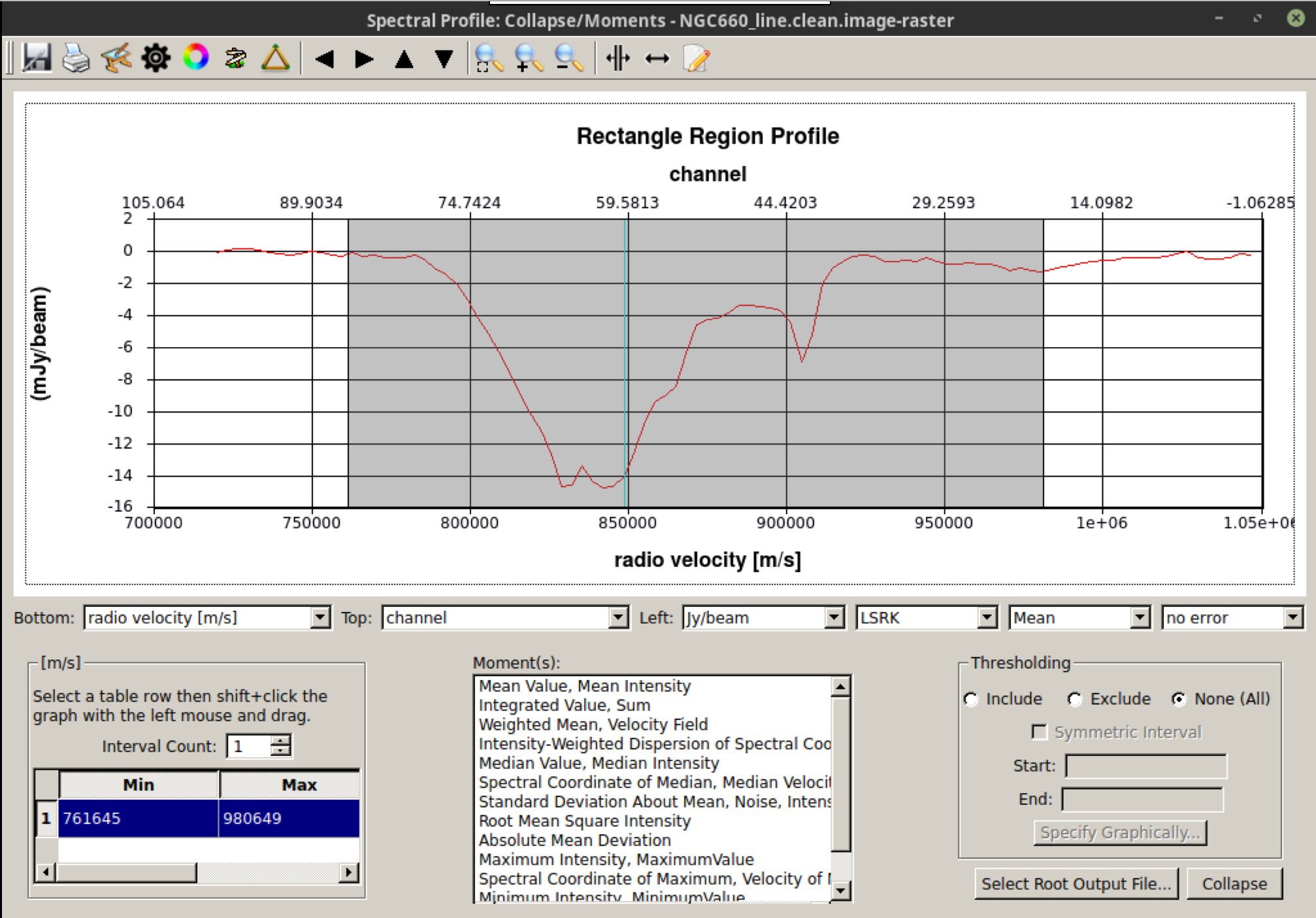
We can also script this using the CASA task immoments, and we should only use the channels that have the line signal.
os.system('rm -rf NGC660line.mom0')
immoments(imagename='NGC660line.image',
		  moments=[0],
		  chans='33~83',
		  outfile='NGC660line.mom0')
When calculating the first moment of the flux-weighted velocity, you need to exclude the noise. Approximately 4 times the rms (see the end of step 9) is suitable for the lower limit, as a negative value; set a high upper limit to exclude since we are only interested in absorption.
os.system('rm -rf NGC660line.mom1')
immoments(imagename='NGC660line.image',
		  moments=[1],
		  chans='33~83',
		  excludepix=[-0.002,1],
		  outfile='NGC660line.mom1')
Open these images in the CARTA viewer and adjust the colour scales to visualize the moment structure.
This shows the zeroth moment and the first moment created using a cutoff of $-0.005\,\mathrm{Jy\,beam^{-1}}$, with some adjustments to the colour scale in Python. You can observe a gradient from blue-shifted on the side of the more prominent NE jet to redshifted towards the weaker counter-jet. This reinforces what we observed when analysing the spectral curve.
B. Extract and plot spectra (step 14)
One of the steps we want to take in our analysis is to observe what the HI absorption spectra look like at different locations across the line of sight. This can provide us with information on the nature of the gas, such as its dynamics.
Load the spectral cube in the viewer/CARTA, select a channel with strong absorption, such as 60, and overplot the continuum contours. (Linux) Click on the spectral profile tool. Draw three ellipses on the core and in the direction of the NE jet and the fainter counter-jet. In practice, you may have additional information to help determine where it is interesting to extract a spectrum. When you click on one of the ellipses, the spectrum will appear in the spectral profile tool. You can also obtain the coordinates (in pixels) from the Region tab.
Scripting uses a tool, ia (for image analysis), to extract the spectra, and then we can use raw Python to create a plot. This would be especially convenient to incorporate into a script for future use.
Define the centres of the three positions; I have set all the radii to 6 pixels (what is that in arcsec?), but they do not have to be the same. This is a Python dictionary, where the keys (e.g., 'jet') are associated with a value that defines each circle.
rgns={'jet':'circle[[156pix, 165pix], 6pix]',
	  'core':'circle[[161pix, 160pix], 6pix]',
	  'cjet':'circle[[167pix, 154pix], 6pix]',
	  'rms':'box[[10pix,10pix],[100pix,50pix]]'}
Use the ia tool to obtain the spectral profile at each of the three positions, along with an off-source noise box, and save them to text files.
ia.open('NGC660_line.clean.image')
for r in rgns:
	outfile=open(r+'.spec', 'w') # create empty text files called 'jet.spec' etc. in writeable mode
	f=ia.getprofile(axis = 3,  # extract the profile and store it in variable f
	                function = 'flux',
	                region = rgns[r],
	                unit='km/s',
	                spectype='radio velocity')
	for z in zip(f['coords'],f['values']): # python to extract the velocity and flux arrays from f in a suitable format
		print >> outfile, z[0], z[1] # print these to the outfile
	outfile.close()

ia.close()
We could have passed the profiles directly to a plotter, but now you have the *.spec files on disk for your use. Let's use Python to plot the spectra.
import matplotlib.pyplot as plt
cols={'jet':'b','core':'g','cjet':'r','rms':'k'} # The colors for each spectrum (use help(plt.colors) for others)
fig = plt.figure(1,figsize=(9,6))
ax = fig.add_subplot(111)
for i in range(len(rgns)):
	v=[];f=[]
	for l in open(list(rgns.keys())[i]+'.spec'):  # Read the disk files back into arrays
		v.append(float(l.split()[0])) # Array of velocities for x-axis
		f.append(float(l.split()[1])) # Array of flux density values for y-axis
	ax.plot(v,f,color=cols[list(rgns.keys())[i]],label=r'%s'%list(rgns.keys())[i])  # Plot the spectra
ax.set_xlabel('Velocity (LSR, km/s)')
ax.set_ylabel('Flux density per channel per 12-mas radius')
ax.set_title('NGC660 HI velocity profiles')
ax.legend() # add the legend to show what each line stands for
fig.savefig('NGC660_HIvelocityprofiles.pdf',bbox_inches='tight') # Write the plot to a pdf
plt.show()
plt.clf()
C. Make an optical depth map (step 15)
The optical depth indicates how much energy has been lost while travelling through a dense medium. This enables us to identify where the obscuration is greatest across the source illuminating this dense medium. In our case, we have our bright continuum superimposed upon the absorption of light by the HI transition. We can use these to calculate the optical depth.
In the optically thin approximation, the optical depth ($\tau$) is defined as $$ \tau = -\ln\left(\frac{|I_L|}{I_C}\right),$$ where $I_L$ represents the flux density of the continuum-subtracted line, and $I_C$ denotes the flux density of the continuum.
This can be done for individual planes of the cube or for an average across multiple planes. Calculate the average of the most intense absorption, such as below half-minimum:
os.system('rm -rf NGC660line.mean')
immoments(imagename='NGC660line.image',
		  moments=[-1],
		  chans='55~69',    # main peak FWHM
		  excludepix=[-0.005,1],
		  outfile='NGC660line.mean')
Expressions like optical depth can be coded in immath:
os.system('rm -rf NGC660.tau')
immath(imagename=['NGC660contap1.image','NGC660line.mean'],
	   mode='evalexpr',
	   expr='-1.*log(-1.*IM1/IM0)',
	   outfile='NGC660.tau')
In viewer/CARTA, adjust the range of values to [0,1] to exclude noise pixels, and you should see something similar to the following:
Hooray, this concludes the spectral line workshop! You have performed self-calibration and imaging of a spectral cube and should have learnt how to remove the continuum emission. In addition, we conducted analysis on the spectral cube using moments, pv maps, and optical depth calculations. This analysis has revealed that the NGC660 outburst consists of two components moving towards and away from the central black hole. Based on the optical depth maps, the obscuring fraction of HI is slightly higher toward the centre of the object, indicating that the gas is denser and could be fueling this outburst.
back to Data Reduction