
Part 1: Basic Calibration
This is the CASA v5 version of this tutorial! If you don't mean to be here, got back to the Data Reduction workshop page to get the CASA v6 tutorials.
Guidance for calibrating EVN data using CASA
This guide uses CASA version 5.7. Important: Before starting, please ensure that the correct version is on your system. On the UNIX command line type casa --nogui to open CASA and look for the following line on the command line and ensure that the highlighted number is equal or larger than 5.7.0 but not CASA version 6+ e.g.:
CASA 5.7.2-4 -- Common Astronomy Software Applications
If you find a version less than 5.7 or 6 or higher, please inform the DARA trainer who can provide the newer version. However, if the version is correct, type exit to exit CASA.
For this workshop, you need about 20 GB of disk space, although one could manage with less by moving early versions of these files to storage.
In the following three parts, we shall build up to making your own calibration scripts by performing the data reduction in three different ways with reducing amount of assistance in each part:
- In Part 1 (this page), we will work interactively to see what each parameter is for. This is used for the initial steps and calibration common to all sources.
- In Part 2, we will calibrate and image one phase-reference and target by entering parameters into a script (
NME_J1849.py). - And finally in Part 3, you shall use the information learnt in the previous sections to generate own calibration script
NME_3C345_skeleton.pyfor the other phase-reference - target pair.
Table of contents
- Data and supporting material
- Data preparation
- The CASA environment
- Data loading and inspection
- Fringe-fitting
- Bandpass calibration
- Apply calibration and split out phase-ref - target pairs
1. Data and supporting material
n14c3 is an EVN network monitoring experiment to see how well the EVN is performing. It contains two target - phase-reference pairs of bright sources (plus a 5th source which we will not use). These data are contained in FITS-IDI files which are output from the correlator. The following table shows the sources in these files we are going to use. Don't worry about knowing what these are going to be used for yet, we will get around to this.
| Number | Name | Position (J2000) | Role |
|---|---|---|---|
| 0 | J1640+3946 | 16:40:29.632770 +39.46.46.02836 | Phase calibrator |
| 1 | 3C345 | 16:42:58.809965 +39.48.36.99402 | Target |
| 2 | J1849+3024 | 18:49:20.103406 +30.24.14.23712 | Target |
| 3 | 1848+283 | 18:50:27.589825 +28.25.13.15523 | Phase calibrator |
| 4 | 2023+336 | 20:25:10.842114 +33.43.00.21435 | Not used |
J1849+3024 is also used as bandpass calibrator because it is a bright, compact source with good data on all baselines. If you are reducing a new data set, you would check the suitability of the bandpass calibrator early in the data reduction process.
For this part, you should have downloaded the tar bundle (EVN_continuum_pt1.tar.gz) using the link on the home page. With this in hand let's start:
- Make a directory called something you will remember, e.g. EVN, and work in it. (Do not do data reduction within the CASA installation).
- Copy the data and files you need to this directory and extract the various scripts using
tar.<path***>is the original location of these files. Note:***means something for you to fill in. e.g:
mkdir EVN
cd EVN
cp <path***>/EVN_continuum_pt1.tar.gz .

tar -xvf EVN_continuum_pt1.tar.gz   # extract the additional material.
- Let's check that all the data is there and we are in the right place. Type
pwdinto the UNIX command line and you should see something like<path***>/EVN/returned (where path is the location which is often the UNIX home). Now typelsinto the command line and you should find at least the following files!
- Raw data (fits IDI files from the JIVE correlator).
n14c3_1_1.IDI1n14c3_1_1.IDI2- Gain curve and $T_\mathrm{sys}$ data file
n14c3.antab- Helper scripts by Mark Kettenis to generate CASA-compatible $T_\mathrm{sys}$ and gain curves from the .antab table.
key.pyappend_tsys.pygc.py- Flag command files. You can write these yourself, but to save time you can use this one.
flagSH.flagcmd- Python script (
NME_all.py.tar.gz) if you get stuck or need to re-calibrate quickly!
2. Data preparation
Now we need to do some pre-calibration using the helper scripts which are provided. The FITS-IDI does not have any extra information on the individual antennas attached such as the system temperatures ($T_\mathrm{sys}$) which provides the flux scaling for the observation nor the gain curves i.e. the difference in the effective sensitivity of the telescopes due to deformation of dishes due to gravity and differing atmospheric opacities with source elevation.
We are going to use CASA in the non-interactive mode and execute the helper scripts. Firstly, we are going to attach the system temperature information to the FITS-IDI files:
casa --nogui -c append_tsys.py n14c3.antab n14c3_1_1.IDI*
The argument -c means that CASA will execute the append_tsys.py file and exit once this is complete. The second argument is the .antab file which contains the $T_\mathrm{sys}$ information and gain information. The final argument selects all of the FITS-IDI files. This will take a few minutes so have a coffee!
Once this is complete, we also need to extract the gain information for each antenna from the antab file. Again we use another script to do this namely gc.py. This will make a CASA table which we shall convert to a gain curve later on (and explain what it does).
casa --nogui -c gc.py n14c3.antab n14c3.gc
This will create the table n14c3.gc.
Now lets fire up CASA in interactive mode!
3. The CASA Environment
To start CASA, we enter the simple command casa into the UNIX command line and should come up with the following:
casa

=========================================
The start-up time of CASA may vary
depending on whether the shared libraries
are cached or not.
=========================================

IPython 5.8.0 -- An enhanced Interactive Python.

CASA 5.7.2-4   -- Common Astronomy Software Applications

Found an existing telemetry logfile: /Users/user/.casa/casastats.log
Telemetry initialized. Telemetry will send anonymized usage statistics to NRAO.
You can disable telemetry by setting environment variable with
export CASA_ENABLE_TELEMETRY=false
or by adding the following line in your ~/.casarc file:
EnableTelemetry: False
--> CrashReporter initialized.
Enter doc('start') for help getting started with CASA...
Using matplotlib backend: TkAgg

CASA <1>:
For those familiar to ipython, this should look similar. Using this prompt, we shall use the various tasks and functions within CASA to begin calibrating our data. In addition, you will see that there is another window opened when we initialised CASA which is the logger. This logger should look something like this:
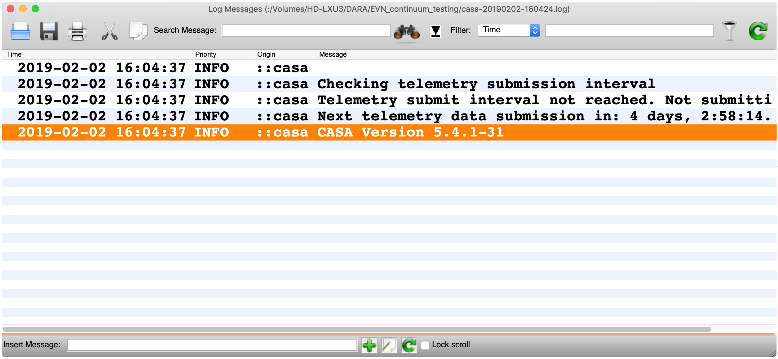
IMPORTANT: The logger will show the information on the tasks which have been executed. It is vitally important to check this to see if there are errors or to evaluate the performance of the calibration. We will use this alot in this tutorial.
4. Data loading and inspection
4A. Load data
Let's use our first task in CASA. Hooray!! We shall be using the importfitsidi task to change the FITS-IDI files (n14c3_1_1.IDI1 & n14c3_1_1.IDI2) we prepared earlier into a CASA compatible format called a measurement set.
Whenever we use a task in CASA (in interactive mode), it is always good practice to make sure that previous inputs are deleted because some inputs are shared across multiple tasks. In the CASA prompt, we can firstly initialise a task using default(<taskname>). So for this purpose we instead type default(importfitsidi) into the prompt.
With the task initialised, we need to set the inputs (explained later) of the task, i.e. what do we want the task to do?. Typing inp() into the prompt should return:
#  importfitsidi :: Convert a FITS-IDI file to a CASA visibility data set
fitsidifile         =       ['']        #  Name(s) of input FITS-IDI file(s)
vis                 =         ''        #  Name of output visibility file (MS)
constobsid          =      False        #  If True, give constant obs ID==0 to the data from all input fitsidi files (False = separate obs id for each file)
scanreindexgap_s    =        0.0        #  min time gap (seconds) between integrations to start a new scan
specframe           =      'GEO'        #  spectral reference frame for all spectral windows in the output MS
So how do we interpret this? The labels to the left of the = are the inputs (e.g. fitsidifile, constobsid, specframe) and the value which they are currently set to are to the right of the =. The default values indicate what sort of input is required (e.g. [''] indicates a string array, False needs a Boolean etc etc.). A short description of each input is given by the text after the hash symbol. To set the inputs we use the syntax <input>=<value/array>. CASA helps here and will colour the input values red if the entry is the wrong data type (as is the case with the fitsidifile input at the moment) and blue if the input is set (i.e. non-default) and is of the right type.
IMPORTANT A key thing to remember when using CASA is the help command. This command gives many more details than the input command and can also provide examples of execution of tasks. Try typing help(importfitsidi) into the command line. This should return something like:
importfitsidi = class importfitsidi_cli_
 |  Methods defined here:
 |
 |  __call__(self, fitsidifile=None, vis=None, constobsid=None, scanreindexgap_s=None, specframe=None)
 |      Convert a FITS-IDI file to a CASA visibility data set
 |
 |              Detailed Description:
 |      Convert a FITS-IDI file to a CASA visiblity data set.
 |
 |              Arguments :
 |                      fitsidifile:    Name(s) of input FITS-IDI file(s)
 |                         Default Value:
 |
 |                      vis:    Name of output visibility file (MS)
 |                         Default Value:
 |
 |                      constobsid:     If True, give constant obs ID==0 to the data from all input fitsidi files (False = separate obs id for each file)
 |                         Default Value: False
 |
 |                      scanreindexgap_s:       min time gap (seconds) between integrations to start a new scan
 |                         Default Value: 0.
 |
 |                      specframe:      spectral reference frame for all spectral windows in the output MS
 |                         Default Value: GEO
 etc etc.
Alternatively you can use the online CASA docs, which provides help for all of these tasks.
Ok lets get back to the importfitsidi task. We want to convert our FITS-IDI files to a visibility file/measurement set. If we look at the inputs, we therefore need to set at least the fitsidifile and the vis inputs. We will also set constobsid and scanreindexgap_s parameters but these are not essential, it just makes the data tidier. Type the following inputs into your CASA prompt:
fitsidifile=['n14c3_1_1.IDI1','n14c3_1_1.IDI2']   # fits files to convert
vis='n14c3.ms'                             # output ms file name
constobsid=True                                   # data could be processed together
scanreindexgap_s=15                               # only separate scans if gap >15 sec (or source change)
Important: After setting your inputs, always check your inputs before running the task. You don't want the task messing up your data! Type inp() again and you'll get the following returned:
CASA <3>: inp
--------> inp()
#  importfitsidi :: Convert a FITS-IDI file to a CASA visibility data set
fitsidifile         = ['n14c3_1_1.IDI1', 'n14c3_1_1.IDI2'] #  Name(s) of input FITS-IDI file(s)
vis                 = 'n14c3.ms' #  Name of output visibility file (MS)
constobsid          =       True        #  If True, give constant obs ID==0 to the data from all input fitsidi files (False = separate obs id for each file)
scanreindexgap_s    =         15        #  min time gap (seconds) between integrations to start a new scan
specframe           =      'GEO'        #  spectral reference frame for all spectral windows in the output MS
As you can see, the inputs which have been set are now blue and the fitsidifile input has changed to blue indicating that the data type is correct. If you are happy with the inputs, the task should be executed by typing either importfitsidi() or go()!.
You will notice that the prompt has gone and nothing can be typed into CASA until the task has finished. Take a look at the logger, this gives you more information into the progress of the task along with what the task is doing and if there are any errors associated with the inputs and/or the data sets.
Once the task is complete, you should find that there is a new file called n14c3.ms. To see this file from within the CASA prompt, you can use an ! before the command to convert it into a UNIX command. For example, typing !ls should return something similar to:
EVN_continuum_pt1.tar.gz  flagSH.flagcmd            n14c3.gc/
NME_all.py.tar.gz         gc.py                     n14c3.ms/
append_tsys.py*           importfitsidi.last        n14c3_1_1.IDI1
casa-20190606-150724.log  key.py                    n14c3_1_1.IDI2
casa-20190606-151817.log  key.pyc
casa-20190606-151918.log  n14c3.antab
One of the most important aspects of data reduction is to understand your data!. Without knowing what your data looks like and its quality, the resultant calibration can often be sub-optimal. CASA provides lots of tools to assess and understand your data. The first, and one of the most essential of these is provided by the listobs task. This task outlines the structure of your data such as the frequencies observed, the antennas involved and the observing plan.
In the CASA prompt, initialise and run listobs using (and remember to check the inputs and what they do using inp() before executing the task):
os.system('rm -rf n14c3.ms.listobs')  # note that this deletes the file that will be made with this task
default(listobs)
vis='n14c3.ms'
listfile='n14c3.ms.listobs'   # This makes a file with the listobs info.
listobs()
The command makes a file in the current working directory called n14c3.ms.listobs which contains information about the measurement set. Try opening this file with your favourite text editor such as gedit. Remember a ! lets you run UNIX commands from CASA. So, if you use gedit, the command to write in the command line would be !gedit n14c3.ms.listobs.
So what is included in this file:
- Scan listings: this shows the pattern of observations. Each scan is about 1 min and each individual integration about 2 sec.
  Date        Timerange (UTC)          Scan  FldId FieldName             nRows       SpwIds           Average Interval(s)
22-Oct-2014/12:00:00.0 - 12:04:00.0     1      1   3C345                 52800  [0,1,2,3,4,5,6,7]  [2, 2, 2, 2, 2, 2, 2, 2]
            12:06:00.0 - 12:10:00.0     2      1   3C345                 63360  [0,1,2,3,4,5,6,7]  [2, 2, 2, 2, 2, 2, 2, 2]
            12:12:00.0 - 12:13:00.0     3      1   3C345                 15840  [0,1,2,3,4,5,6,7]  [2, 2, 2, 2, 2, 2, 2, 2]
            12:13:40.0 - 12:14:40.0     4      1   3C345                 15840  [0,1,2,3,4,5,6,7]  [2, 2, 2, 2, 2, 2, 2, 2]
            12:15:20.0 - 12:16:20.0     5      0   J1640+3946            15840  [0,1,2,3,4,5,6,7]  [2, 2, 2, 2, 2, 2, 2, 2]
            12:17:00.0 - 12:18:00.0     6      1   3C345                 13200  [0,1,2,3,4,5,6,7]  [2, 2, 2, 2, 2, 2, 2, 2]
            12:18:40.0 - 12:19:40.0     7      0   J1640+3946            13200  [0,1,2,3,4,5,6,7]  [2, 2, 2, 2, 2, 2, 2, 2]
            12:20:20.0 - 12:21:20.0     8      1   3C345                 15840  [0,1,2,3,4,5,6,7]  [2, 2, 2, 2, 2, 2, 2, 2]
.......
- Names and positions of fields observed.
Fields: 5
ID   Code Name                RA               Decl           Epoch        nRows
0         J1640+3946          16:40:29.632770 +39.46.46.02836 J2000       254400
1         3C345               16:42:58.809965 +39.48.36.99402 J2000       383520
2         J1849+3024          18:49:20.103406 +30.24.14.23712 J2000       276480
3         1848+283            18:50:27.589825 +28.25.13.15523 J2000       388800
4         2023+336            20:25:10.842114 +33.43.00.21435 J2000       542880
- Correlator set-up: there are 8 spectral windows (or IFs), each of 32 channels, and 4 polarisation products (we will only use the total intensity combination of RR and LL).
Spectral Windows:  (8 unique spectral windows and 1 unique polarization setups)
SpwID  Name   #Chans   Frame   Ch0(MHz)  ChanWid(kHz)  TotBW(kHz) CtrFreq(MHz)  Corrs
0      none      32    GEO    4926.990       500.000     16000.0   4934.7400   RR  RL  LR  LL
1      none      32    GEO    4942.490       500.000     16000.0   4950.2400   RR  RL  LR  LL
2      none      32    GEO    4958.990       500.000     16000.0   4966.7400   RR  RL  LR  LL
3      none      32    GEO    4974.490       500.000     16000.0   4982.2400   RR  RL  LR  LL
4      none      32    GEO    4990.990       500.000     16000.0   4998.7400   RR  RL  LR  LL
5      none      32    GEO    5006.490       500.000     16000.0   5014.2400   RR  RL  LR  LL
6      none      32    GEO    5022.990       500.000     16000.0   5030.7400   RR  RL  LR  LL
7      none      32    GEO    5038.490       500.000     16000.0   5046.2400   RR  RL  LR  LL
- Antennas used. The offset from the array centre is zero since the absolute Earth-centred (geocentric) coordinates are given for each antenna.
Antennas: 12:
ID   Name  Station   Diam.    Long.         Lat.                Offset from array center (m)                ITRF Geocentric coordinates (m)
                                                                   East         North     Elevation               x               y               z
0    EF    EF        0.0  m   +006.53.01.0  +50.20.09.1          0.0000        0.0000  6365855.3595  4033947.234200   486990.818800  4900431.012900
1    WB    WB        0.0  m   +006.38.00.0  +52.43.48.0          0.0000        0.0000  6364640.6582  3828445.418100   445223.903400  5064921.723400
2    JB    JB        0.0  m   -002.18.30.9  +53.03.06.6         -0.0000        0.0000  6364633.4245  3822625.831700  -154105.346600  5086486.205800
3    ON    ON        0.0  m   +011.55.04.0  +57.13.05.3          0.0000        0.0000  6363057.6347  3370965.885800   711466.227900  5349664.219900
4    NT    NT        0.0  m   +014.59.20.6  +36.41.29.4          0.0000        0.0000  6370620.8444  4934562.806300  1321201.578200  3806484.762100
...
4B. Correct antenna tables
As you may have noticed, the antenna information in the listobs output showed that the antennas have no diameters nor any axis offsets. In the future, this will be supplemented by a separate CASA task but we have to insert it manually at the moment. This is not vitally important to remember so it may be easier to just copy and paste the following commands into the CASA prompt:
# Copy these arrays of values (no line breaks in each array)
ants=  ['EF','WB','JB','ON','NT','TR','SV','ZC','BD','SH','HH','YS','JD']
diams= [100.0,300.0,75.0,25.0,32.0,32.0,32.0,32.0,32.0,25.0,24.0,40.0,25.0]
axoffs=[[0.013,4.95,0.,2.15,1.831,0.,-0.007,-0.008,-0.004,-0.002,6.692,2.005,0.]
,[0.,0.,0.,0.,0.,0.,0.,0.,0.,0.,0.,0.,0.]
,[0.,0.,0.,0.,0.,0.,0.,0.,0.,0.,0.,0.,0.]]

# Modify the antenna table
tb.open('n14c3.ms/ANTENNA', nomodify=False)
tb.putcol('DISH_DIAMETER', diams)
tb.putcol('OFFSET',axoffs)
tb.close()
Run a listobs (listobs(vis='n14c3.ms')) and check the logger and to ensure that these have been updated accordingly! Note that we will use what we call a reference antenna later for calibration. This is normally chosen as the most sensitive antenna in the array, hence this will be Effelsberg (EF).
4C. A priori calibration
If you remember earlier, the append_tsys.py helper script was used to attach the system temperature information for each telescope to the FITS-IDI files. The system temperature is measured every few minutes. This compensates roughly for the different levels of signal from different sources, the effects of elevation and other amplitude fluctuations. Each antenna has a characteristic response in terms of Kelvin of system temperature per Jy of flux, so $T_\mathrm{sys}$ is also used to scale the flux density.
In CASA, calibration is conducted using calibration tables which are then used to modify the visibilities. To obtain our fluxscaling we therefore have to generate a system temperature calibration table using the task gencal. This task is used to generate caltables from ancillary information which can be found in the measurement set or in external files, and can also be used to create manual calibration tables from scratch. The gencal task has a special function to generate $T_\mathrm{sys}$ tables. To generate these tables we need to input:
# In CASA
default(gencal)  # This reads the Tsys information appended to a ms
vis='n14c3.ms'
caltable='n14c3.tsys'
caltype='tsys'
uniform=False   #Set to False to get spw dependent Tsys extraction
gencal()
You will find that there is a new table named n14c3.tsys which contains the gain information.
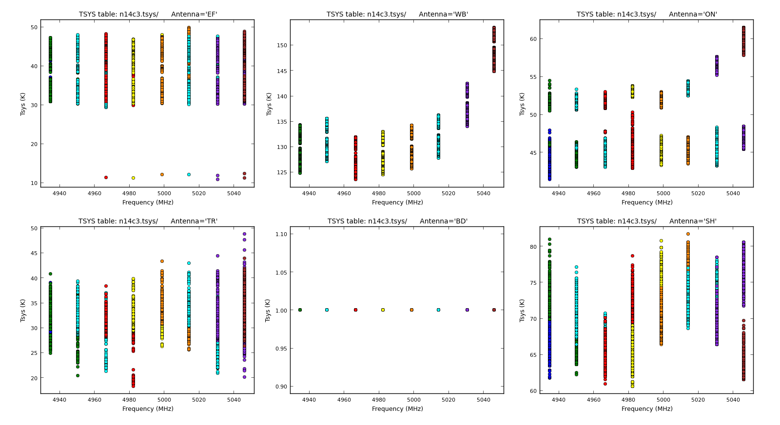
Important: A key factor whenever generating calibration tables is to inspect them to see if there are errant values which simply do not make sense. To inspect tables, we can use either plotcal or, since CASA v5.4, plotms. For this example, we shall use plotcal. If we initialise the task (remember use default), we can see that we have to set the $x$ and $y$ axes along with what each plot shall be iterated over. So in this case we want to plot $T_\mathrm{sys}$ against frequency for each antenna. Note that the subplot parameter is the matplotlib subplot syntax. We should therefore input the following:
default(plotcal)
caltable='n14c3.tsys'
xaxis='freq'
yaxis='tsys'
subplot=321
iteration='antenna'
plotcal()
This should give an output similar to:
Note that the next button in the GUI will iterate and show 2nd batch of 6 antennas. We can also see how the $T_\mathrm{sys}$ changes over time! Most parameters are already set from the last run of plotcal, therefore we can just write (and remembering to check the inputs before running!):
xaxis='time'
inp()
plotcal()
This should generate a plot similar to:
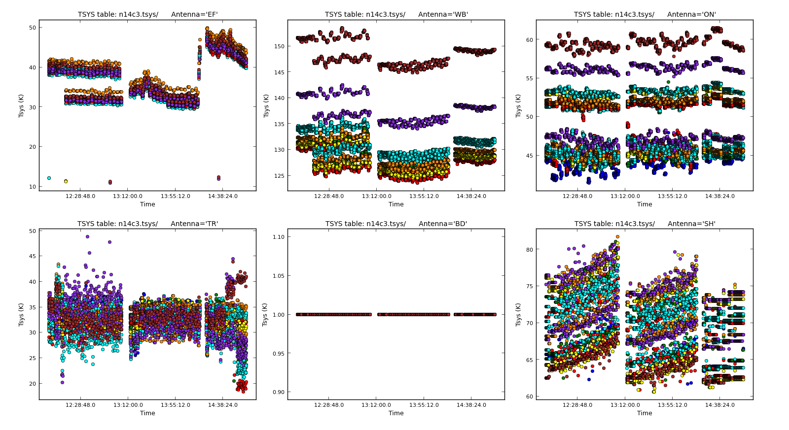
You can see the changes with each source change.
Three antennas do not have $T_\mathrm{sys}$ measurements, but in the next step we will generate the gain curve table. This provides the scaled gain-elevation correction which scales the visibility amplitudes to the sensitivity of the dish, albeit without any allowance for weather or source contributions. Again, we use gencal to do this and the gain information (n14c3.gc) that we extracted from the .antab file:
# In CASA
default(gencal)
vis="n14c3.ms"
caltable= "n14c3.gcal" ## Name of output gain curve cal. table
caltype="gc"           ## Special caltype for gaincurves
infile="n14c3.gc"      ## Gaincurve information derived from antab file

gencal()
4D. Inspect and flag data
One of the most important aspects of radio interferometric data reduction is identifying and removing bad data. As you will see in the lectures, often these bad data is due to Radio Frequency Interference (RFI) from satellites and mobile phones, however sometimes it can be many other factors such as correlation errors or antennas off source. While it sounds tedious, the effects of bad data can be significant if ignored therefore careful extraction and removal of bad data is of paramount importance. In this sub-section, we shall inspect our visibilities and attempt to flag and remove bad data.
- To begin, we shall remove the autocorrelations as these are not useful for continuum interferometric observations. To do this we use the manual flagging task called
flagdata. Take a look at the inputs. To flag all of the autocorrelations we simply leave all as default (i.e. all data is selected) and set theautocorrparameter to be True
# In CASA
default(flagdata)
vis='n14c3.ms'
mode='manual'
autocorr=True

flagdata()
- Next we can see what telescopes are involved and their position relative to each other are using the CASA task
plotants.
# In CASA
default(plotants)
vis='n14c3.ms'

plotants()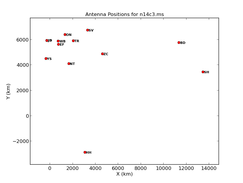
- To inspect the quality of the data, we are going to use the task
plotmsto look for bad data. We start by looking at a bright source where it is easiest to tell good and bad data apart. Theplotmstask is very complicated (take a look at the inputs of the task) and takes a little while to understand. We are going to look at the frequency axes first (so we can average the time axes!) and look at the baselines to the most sensitive telescope (which is the 100m Effelsberg dish).
# In CASA
default(plotms)
vis='n14c3.ms'
xaxis='frequency'
yaxis='amp'
field='1848+283'        # The phase-cal/bandpass cal
avgtime='3600'          # Will only average within scans unless additionally told to average scans too
antenna='EF&*'          # Plot all baselines to the largest and most sensitive antenna
correlation='RR,LL'     # Only plot the parallel hands; the cross hands are fainter (and we won't be using them).
coloraxis='antenna2'

plotms()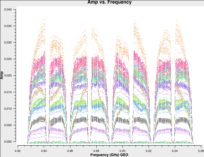
- You can change the plot interactively in plotms.
- You can see 8 spw; the edges of this have low amplitudes due to poor sensitivity and there are some data all at zero.
- Zoom in (using
 ) and use select to highlight bad data (
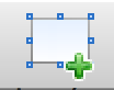 ) and use locate (
 ) to see what antenna it is associated with.
 - You should see that this is mostly on antenna SV (Svetloe; dark green in this plot).
flagdata can make an automatic backup but it will not have a memorable name). The backups for this data set are stored in n14c3.ms.flagversions. We will now back up the flags for this data set now using the task flagmanager. The same task can be used to revert back to old flags too!:
# In CASA
default(flagmanager)
vis='n14c3.ms'
mode='save'           # This mode saves the current flags, use the mode restore to revert to old flagging versions
versionname='preSVandEndChans'  # This is the version name, you can see all version names in flagversions by using mode='list'
flagmanager()
- Now that we have identified that the SV telescope is not working properly, we can flag the telescopes using the
flagdatatask that we used earlier.
# In CASA
default(flagdata)
vis='n14c3.ms'
mode='manual'
antenna='SV'
go()
- Now we should re-inspect the data for any more corrupted data. Plot the most sensitive baseline to see the end channels more clearly and note which are below about half the maximum amplitude. These cause issues further down the line if not flagged and do not contribute much to the final image sensitivity.
# In CASA
default(plotms)
vis='n14c3.ms'
xaxis='channel'
yaxis='amp'
field='1848+283'        # The phase-cal/bandpass cal
avgtime='3600'          # Will only average within scans unless additionally told to average scans too
antenna='EF&JB'          # Plot the baseline of largest and most sensitive antennas
correlation='RR,LL'     # Only plot the parallel hands; the cross hands are fainter (and we won't be using them).
iteraxis='spw'

plotms()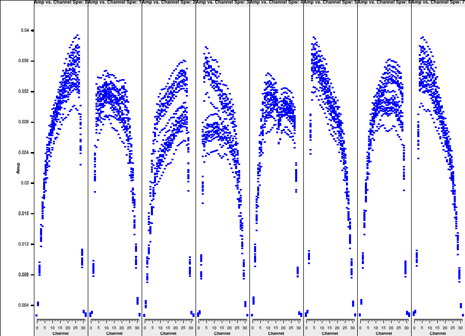
- Use the arrows at the bottom of
plotmsto scroll through the spw (which should got through the subplots above). Odd and even spw behave differently but there is no need to spend too much time on this as the suggested channels to flag are given here for time saving purposes:
# In CASA
default(flagdata)
vis='n14c3.ms'
mode='manual'
spw='0:0~5;29~31,2:0~5;29~31,4:0~5;29~31,6:0~5;29~31,1:0~2;27~31,3:0~2;27~31,5:0~2;27~31,7:0~2;27~31'

flagdata()
We can see whether this has worked by pressing reload in the plotms window and plot the same again. These edge channels should now have disappeared.
- Next we shall look at amp vs. time instead, now averaging in frequency:
# In CASA
default(plotms)
vis='n14c3.ms'
xaxis='time'
yaxis='amp'
field='1848+283'
spw='0~7:13~20'        # Average a few central channels where the response is stable
avgchannel='8'
antenna='EF&*'
correlation='RR,LL'
coloraxis='baseline'

plotms()
- Note that the first one or two integrations of some scans are bad. There is a specific
flagdatamode for this called quack. We will safely assume that all sources are affected.
# In CASA
default(flagdata)
vis='n14c3.ms'
mode='quack'
quackinterval = 5     # 5 seconds, or just over 2 intgrations

flagdata()
- Now go through each baseline to identify remaining bad data (enter
iteration='baseline'and re-loadplotms). Again, this has already been listed so don't spend too long, just make sure you have some idea of how to identify and record bad data. There is more than one bad scan on HH and as we are plotting the phase-cal it is likely that the target in-between was affected. Plot this.
# In CASA
default(plotms)

vis='n14c3.ms'
xaxis='time'
yaxis='amp'
scan='60~70'            # a few scans including the bad data; plot all fields in this time range
spw='0~7:13~20'
avgchannel='8'
antenna='EF&HH'         # just the relevant baseline
correlation='RR,LL'
coloraxis='field'       # distinguish sources

plotms()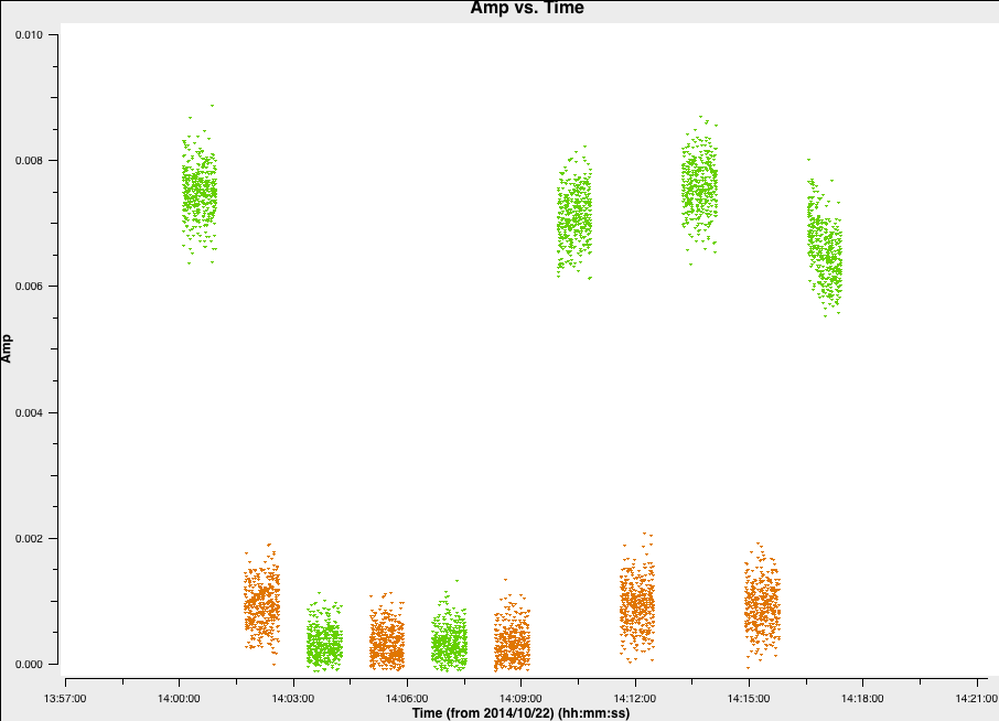
- Flag the scans when the target (in brown in the plot here) goes right to zero. Or for time-saving purposes we have put the commands in here for you.
# In CASA
default(flagdata)
vis='n14c3.ms'
antenna='HH'
mode='manual'
scan='62~65'

flagdata()
- Next, lets inspect the next most distant antenna, SH
# In CASA
default(plotms)

vis='n14c3.ms'
xaxis='time'
yaxis='amp'
field='1848+283'
spw='0~7:13~20'
avgchannel='8'
antenna='EF&SH'         # just the relevant baseline
correlation='RR,LL'
coloraxis='spw'         # distinguish spw

plotms()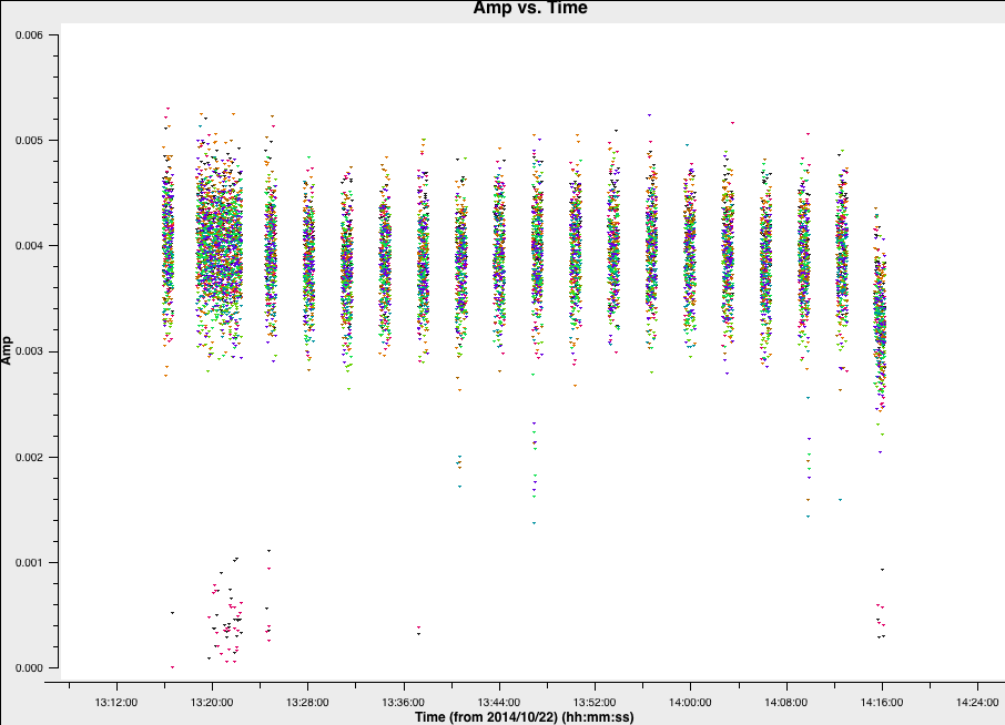
There are many short, bad periods, some only affecting certain spw. The easiest way to cope with this is to write a flag list. Identify antennas/spw/times, adding 1s to the start and finish of each flagging period. They are all shorter than one scan so the same flags aren't applied to the target but later, we will look for similar bad data on the target. Take a look at the flag list file: flagSH.flagcmd which is in your current directory and cross-check that these entered values are affected.
If you are happy, then we will use this file to automatically flag those channels specified in the file:
# In CASA
default(flagdata)
vis='n14c3.ms'
mode='list'
inpfile='flagSH.flagcmd'

flagdata()
Let's reinspect to check that the bad data are all gone:
# In CASA
default(plotms)
vis='n14c3.ms'
xaxis='time'
yaxis='amp'
field='1848+283'
spw='0~7:13~20'
avgchannel='8'
antenna='EF&*'
coloraxis='corr'
correlation='RR,LL'

plotms()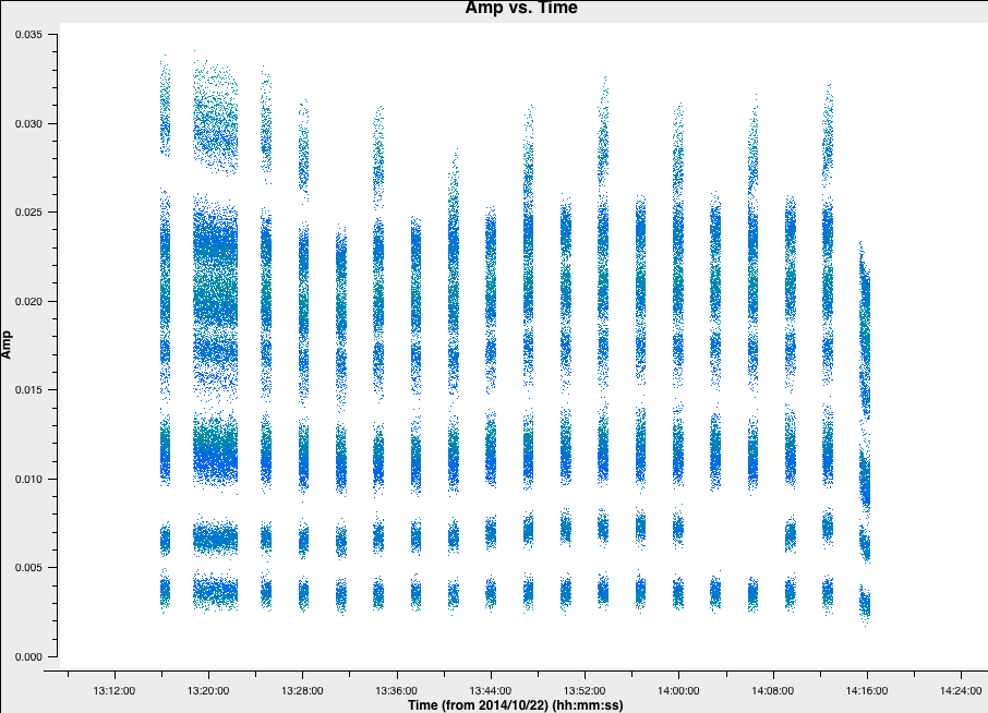
Hooray, the data looks clean! We can finally begin to calibrate these data!
5. Fringe fitting
Now that all the data has been cleaned up, we can begin to think about calibrating these data. As you may remember from the accompanying lectures, the wavefronts arriving at two different telescopes from a single source arrives at different times, i.e. one signal is delayed relative to each other. This is shown by the $D\sin(\theta)$ term in the two-element interferometer shown below:
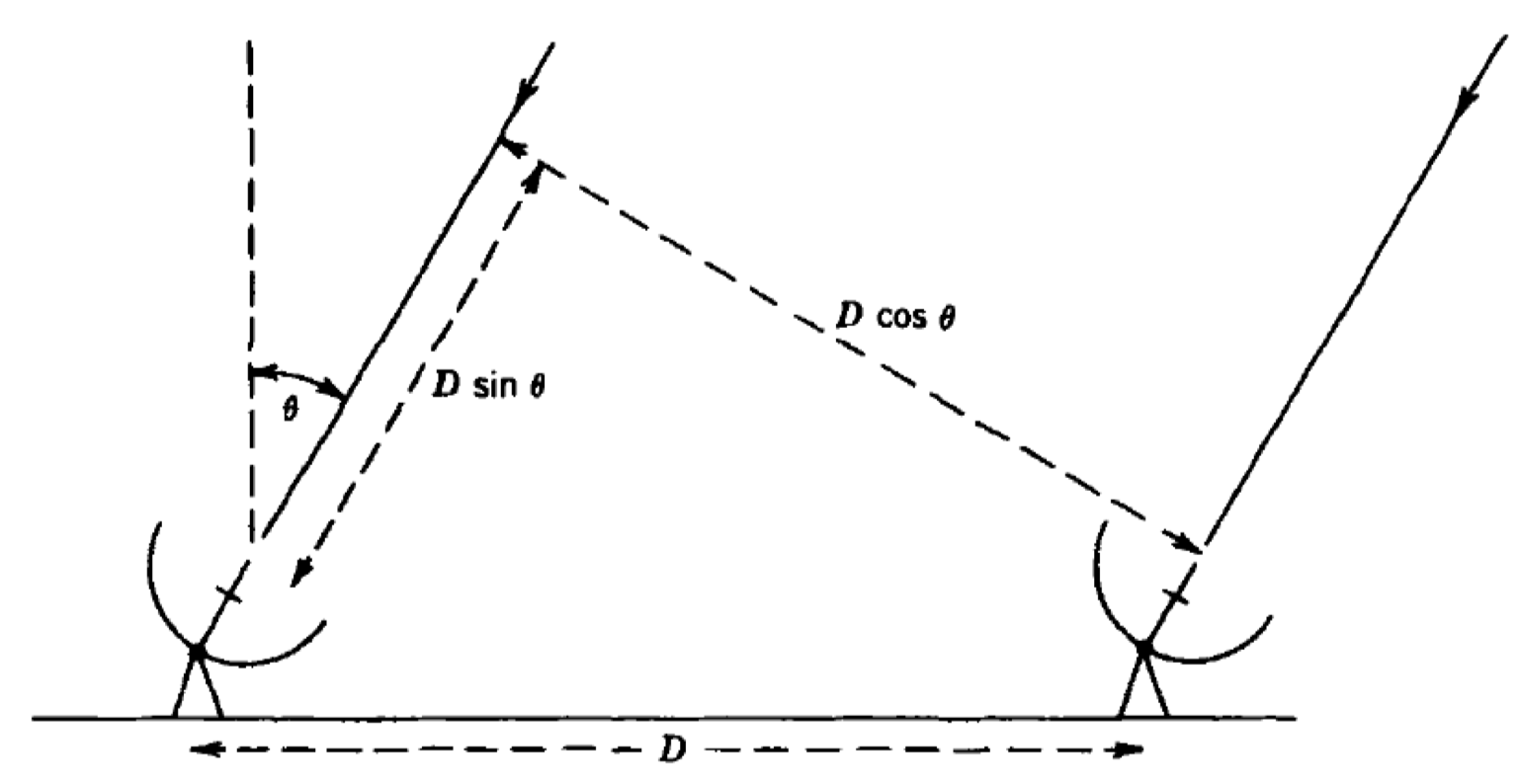
The actual delay term, $\tau_\mathrm{obs} = (D/c)\sin(\theta)$ changes with time because the source position relative to the baseline changes. This means that the interferometer phase ($\phi=2\pi\nu\tau_\mathrm{obs}$) also changes with time giving rise to what we call fringe rates!. The correlator normally corrects for $\tau_\mathrm{obs}$ using a model which is sufficient for small baseline, connected arrays but not for VLBI.
These residual phase, delay and rate errors due are mainly due to atmospheric fluctuations and residuals from the geometric delay compensation by the correlator. As the phase ($\phi$) is related to the delay ($\tau_\mathrm{obs}$), the phase error will depend on the delay error!. To solve for the phase error ($\Delta\phi$) we assume a linear phase model for each antenna i.e. $$\Delta\phi(t,\nu)=\phi_{0} + \left(\frac{\partial\phi}{\partial\nu}\Delta\nu + \frac{\partial\phi}{\partial t}\Delta t\right)$$ where $\phi_{0}$ is the phase error at the reference time and frequency, $\frac{\partial\phi}{\partial\nu}\Delta\nu$ is the delay and $\frac{\partial\phi}{\partial t}\Delta t$ is the rate term. Therefore for a baseline with antennas $i$ and $j$, the relative phase error, $\Delta\phi(t,\nu)_{ij}$ can be modelled as $$\Delta\phi(t,\nu)_{ij}=\phi_{0i} - \phi_{0j} + \left(\left[\frac{\partial\phi_i}{\partial\nu}-\frac{\partial\phi_j}{\partial\nu}\right]\Delta\nu + \left[\frac{\partial\phi_i}{\partial t} - \frac{\partial\phi_j}{\partial t}\right]\Delta t\right).$$ In the following section, we are going to attempt to solve this equation by using all of the baselines to estimate the phase delay and rates relative to some reference antenna. Remember that the interferometer is sensitive to differences therefore the relative phases, delays and rates need to be corrected, not the absolute!
5A. Instrumental Delays
Some of the errors in the aforementioned equation originates from instrumental effects. In systems where different spectral windows have different electronics, the signal chain itself can introduce delays. This can be thought of as the signal at different frequencies travelling different lengths of cable. These delays are mostly constant across the observation time (the residuals are corrected later), therefore we can use a small chunk of data to estimate these (on timescales < the change of delay induced by the atmosphere). Let's plot a small chunk of data to show these delays:
# In CASA
default(plotms)
vis='n14c3.ms'
xaxis='frequency'
yaxis='phase',
ydatacolumn='data'
antenna="EF"
correlation='ll'
coloraxis='baseline'
timerange='13:53:20.0~13:54:20.0'
averagedata=True
avgtime='120'
plotms()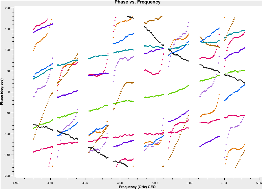
You can see that the instrumental delays show as jumps in phase between the spectral windows. If you notice, we are using a small timerange (~4 mins) on a bright source (1848+283) because, in order to characterise these jumps, we need a high S/N on each spectral window.
To correct these instrumental delays, we are going to use the fringefit task which is new since CASA v5.3. This solves the above equation in order to eliminate the phase errors with respect to time and frequency. Important The CASA calibration routines will assume that the source you are using is a point source at the center of the field (this means the amplitude of this source is the same on all baselines and phases are equal to zero!). Phase calibrators are normally chosen so that the majority of flux is in a point-like component so this initial assumption is valid. We shall refine this in part 2!
# In CASA
default(fringefit)
vis="n14c3.ms"
caltable= "n14c3.sbd"
timerange='13:53:20.0~13:54:20.0'
solint='inf'
zerorates=True
refant='EF'
minsnr=50
gaintable=['n14c3.gcal', 'n14c3.tsys']
interp=['nearest','nearest,nearest']
parang=True

fringefit()
Note that the rates are set to zero. The key thing here is that the instrumental delay calibration aims to correct for differences in signal paths between the spectral windows at individual antennas. We assume these are constant over the experiment and so we apply this solution to the whole observation. If we allow non-zero rates the application of this calibration would extrapolate their effects across the whole experiment, and the term linear in time would dominate the correction far away from the time used to calculate the correction.
The fringefit task reports the signal to noise ratio for each station, as well as the number of iterations it requires to converge on a solution. These are good estimates of how the task performs. For this dataset the signal to noise is very high, and the number of iterations is of the order 10 or less.
In most CASA calibration steps, as above, we feed the new calibration task a list of calibration tables to be applied on the fly while calculating the solutions. However, for the plotms task this is not the case and the calibration solutions have to be applied. In this mind, it is therefore useful to now introduce you to the applycal task which uses these calibrations tables you have derived in order to modify the visibilities.
In the CASA framework, the applycal task takes the DATA column in the measurement set (which contains the visibilities), copies these into the CORRECTED_DATA column and then adjusts this copy using the various calibration tables derived. In this case, we want to apply all tables derived so far i.e. n14c3.tsys, n14c3.gcal, n14c3.sbd to these data.
Take a look at the inputs of applycal and you should see that these are the parameters we should set:
# In CASA
default(applycal)
vis='n14c3.ms'
gaintable=['n14c3.gcal', 'n14c3.tsys', 'n14c3.sbd']
interp=['nearest','nearest,nearest','nearest']
parang=True

applycal()
Note that you may get the error message ..ant=12 cannot be calibrated by n14c3.tsys as mapped, and will be flagged.. can be safely ignored. There were no observations by this telescope hence the applycal will remove this. With the calibration applied, we can see how the instrumental delay calibration has adjusted our data. To do this, we can use the same parameters in plotms as before but instead plot the CORRECTED_DATA column instead. Important: We can cheat a little here because CASA saves the last set of parameters into a file with suffix .last (try typing !ls into the CASA prompt). To load this file and the last set of parameters we use the command tget(<task name>).
In this case, you should type tget(plotms) and type inp to see that the inputs from the last execution of the task is there. As you may identify, we only need to change one parameter i.e. the ydatacolumn from 'data' to 'corrected'. Run plotms and you should see the following:
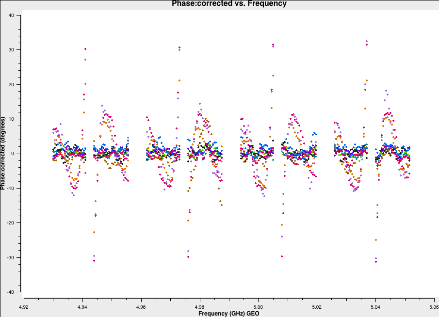
As you can see the phases are flattened, which is good. If we try a different timerange though (we have used a timerange of 13:18:00~13:20:00 in the below plot) the phases still have slopes across the data but the jumps between the spectral windows have been removed. The removal of these jumps means that we can now merge the spectral windows which gives up a much larger S/N to play with. This is what we are going to do in the next section.
5B. Multi-band delays
In the next steps, we are now going to combine the spectral windows in order to get multi-band delays and track the change in the delay signal across the observation. This essentially solves the full phase equation and derives phase, delay and rate corrections for all antennas relative to a reference antenna.
To do this, we need to use the combine input of the fringefit task in order to use all spectral windows at once and we are going to set the averaging time (or solution interval) to 60s. The choice of solution interval should be set so that you have enough S/N to get good solutions, but short enough timescales in order to track the changes in the delays, rates and phases. Note that because one of our phase calibrators (1848+283) is very bright, we can use it to derive the instrumental delays AND the time-dependent delays. In standard VLBI observations there are scans of very bright sources which are used as fringe finders for correlation. These are then also used to derive the instrumental delays (remember that for instrumental delays, we have to have high S/N in each spectral window so the source needs to be very bright!).
After this, we would then use the phase calibrator as the time-dependent delay, phase and rate calibrator. This also takes into account the phase differences induced by the atmosphere over the course of the observation. A key premise of our phase calibrator selection is that these sources should be located near to the target source. This means that we can assume that the solutions derived over time for the phase calibrator is approximately correct for the target field seen as the signal path through the atmosphere is similar. The instrumental delay calibrator does not need to be close to the target field simply because we are correcting for delays induced by instrumental differences which is almost irrespective of the pointing direction of the antennas.
Lets do the multi-band fringe fitting. Note that we have two phase calibrators (1848+283 and J1640+3946), so to save time we are going to conduct the initial fringe fitting on both of these calibrators.
# In CASA
default(fringefit)
vis="n14c3.ms"
caltable= "n14c3.mbd"
field='1848+283,J1640+3946'
solint='60s'
zerorates=False
refant='EF'
combine='spw'
minsnr=30
gaintable=['n14c3.gcal', 'n14c3.tsys','n14c3.sbd']
interp=['nearest','nearest,nearest','nearest']
parang=True

fringefit()
This step may take a while depending on the spec. of your computer so go get a coffee. The S/N parameter needs to be set carefully such that we don't pass erroneous solutions. In this experiment all of the phase calibrators are bright so a high S/N, like 30 as used here, is ok. However, many phase calibrators are not this strong so a S/N threshold of 5 or even 3 may have to be used in order to converge on enough good solutions.
Obtaining good solutions is often trial and error. However, here are some tips in order to assess whether your solutions are good:
- The phases, rates and delays should be smoothly varying if the solutions are good. If the solutions look like noise (with large ranges!) then you may need to increase the averaging interval or the S/N threshold. However, you do not want to increase the S/N so high such that solutions cannot converge.
- CASA will tell you how many solutions fail in the logger. Note that by default CASA will then flag the ranges where solutions fail when the calibration tables are applied. This is an easy way to flag all of your good data! Typically around 5% or less failed solutions are ok!
2019-02-08 12:03:06	INFO	fringefit::::	Calibration solve statistics per spw:  (expected/attempted/succeeded):
2019-02-08 12:03:06	INFO	fringefit::::	  Spw 0: 38/38/38
2019-02-08 12:03:06	INFO	fringefit::::	  Spw 1: 0/0/0
2019-02-08 12:03:06	INFO	fringefit::::	  Spw 2: 0/0/0
2019-02-08 12:03:06	INFO	fringefit::::	  Spw 3: 0/0/0
2019-02-08 12:03:06	INFO	fringefit::::	  Spw 4: 0/0/0
2019-02-08 12:03:06	INFO	fringefit::::	  Spw 5: 0/0/0
2019-02-08 12:03:06	INFO	fringefit::::	  Spw 6: 0/0/0
2019-02-08 12:03:06	INFO	fringefit::::	  Spw 7: 0/0/0
2019-02-08 12:03:07	INFO	fringefit::::	##### End Task: fringefit            #####
2019-02-08 12:03:07	INFO	fringefit::::+	##########################################
You can see that all of the solutions are contained in spectral window 0 (spw). This is because we have combined the spws and so CASA puts the solutions into the first spw for book-keeping. This means that we will have to manually specify which spws these solutions are applied to later. You can also see that CASA has attempted 38 solutions and succeeded on all solutions! This is the first good indicator that the solutions are good.
Next, we need to ensure these solutions are good by inspecting the calibration table. The fringe-fitter solves for delay, phases and rates so we should check all of these. We will firstly check the delays.
# In CASA
default(plotcal)
caltable='n14c3.mbd'
yaxis='delay'
xaxis='time'
iteration='antenna'
subplot=321
plotcal()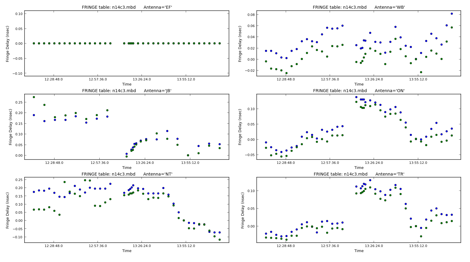
You can see the delays are mostly smoothly varying in time which indicates that the solutions for both phase calibrators are good!. Also, note that EF is zero because this is the reference antenna and the delays are measured relative to this antenna. Next we should check the phase solutions. We shall just use the tget command again as you only need to change one parameter in plotcal:
# In CASA
tget(plotcal)
yaxis='phase'
go()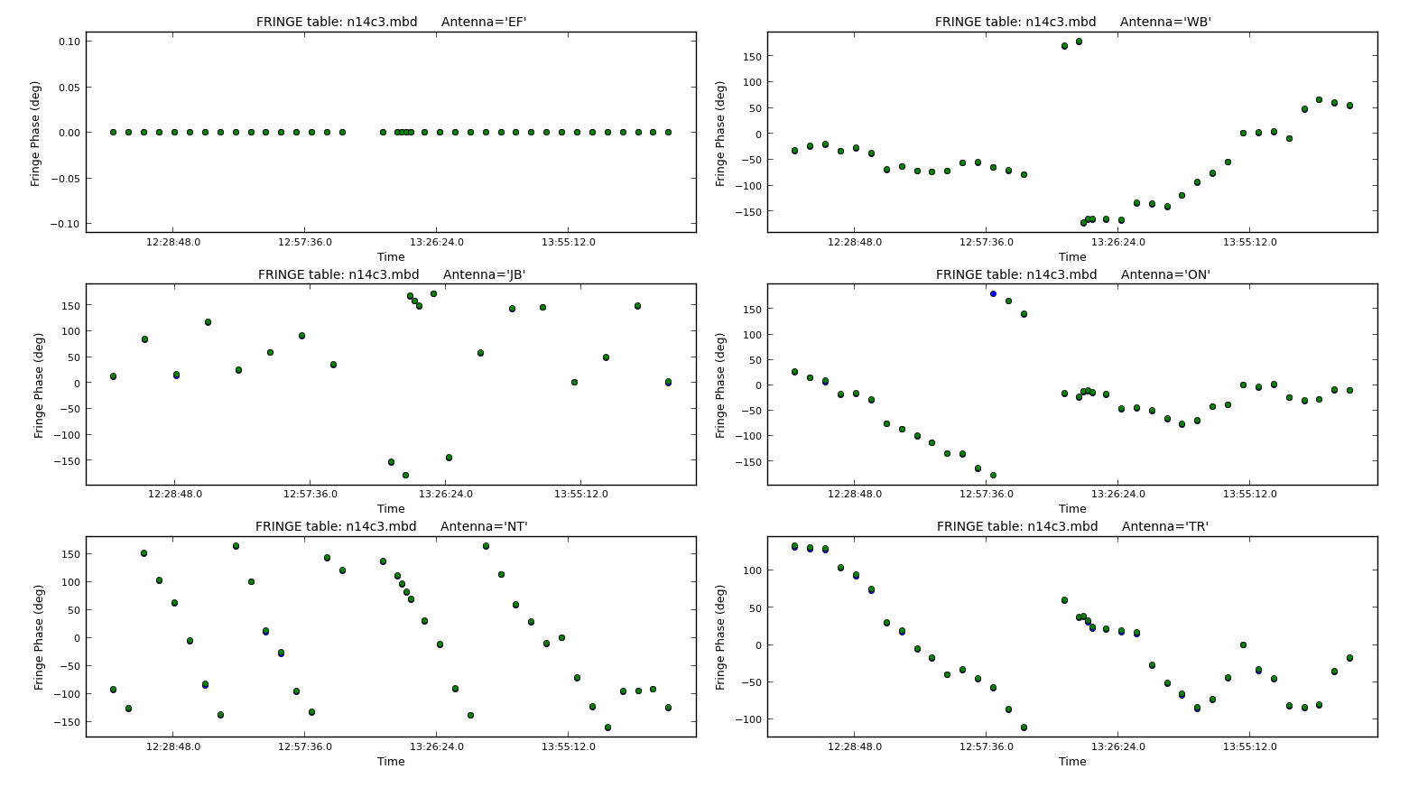
These also change smoothly in time (mostly!) so we can be happy with these. Finally, let's check rates (I'll let you work out how to plot this):
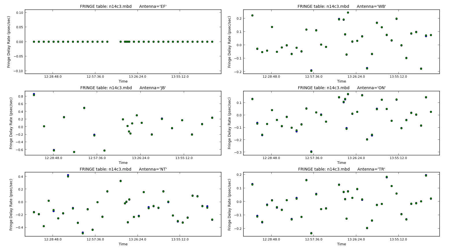
These solutions are a little noisier but note that the scale is much smaller. This should also be ok. Let's apply these solutions so that we can view the results. Note that because we apply these solutions to our target fields, we want to linearly interpolate the multi-band fringe fitting seen as the correct phases/delays/rates for the target field is going to be in between the two phase calibrator scans surrounding it.
default(applycal)
vis="n14c3.ms"
field="1848+283,J1849+3024"
gaintable=["n14c3.tsys", "n14c3.gcal", "n14c3.sbd", "n14c3.mbd"]
interp=['nearest','nearest,nearest','nearest','linear']
spwmap=[[], [], [], 8*[0]]
parang=True
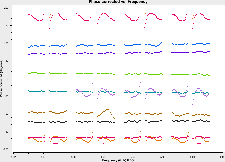
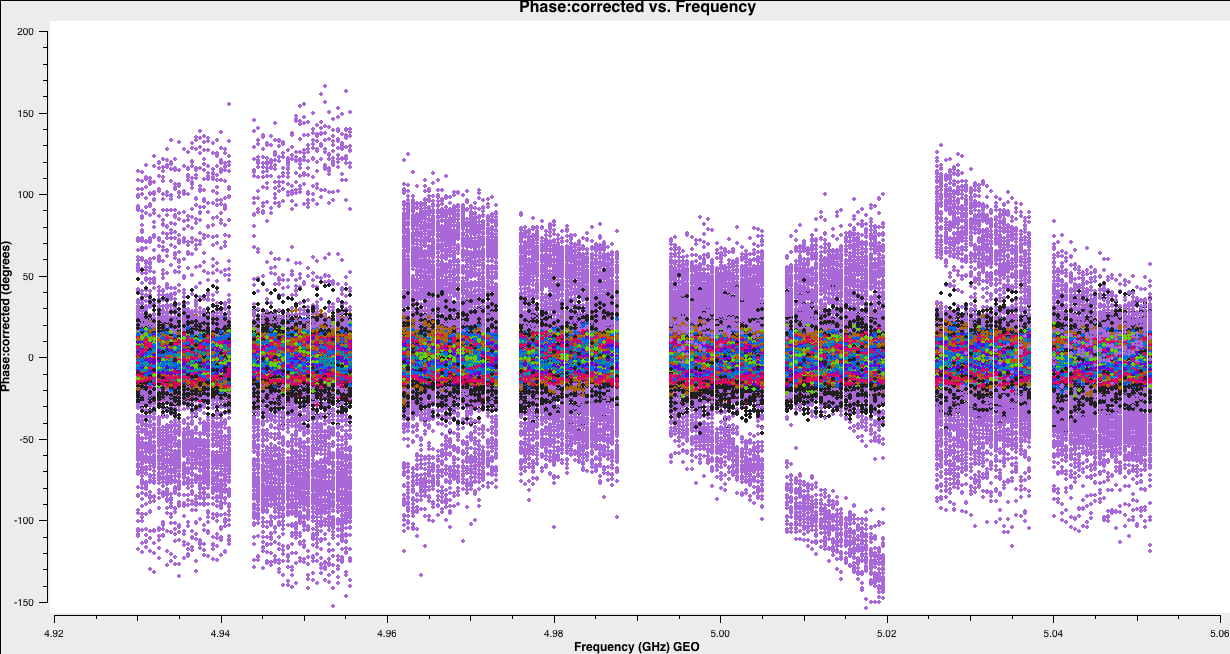
applycal()And let's see our phases on each baseline as a function of frequency on the original scan used to calculate the instrumental delay:
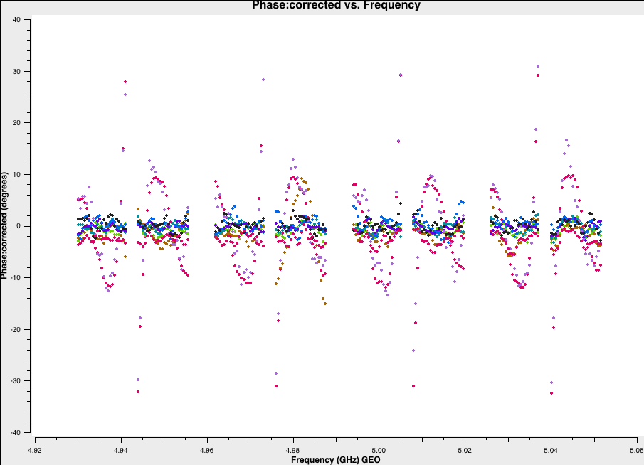
And for the other scan where the baseline phases were offset with just the instrumental delay applied:
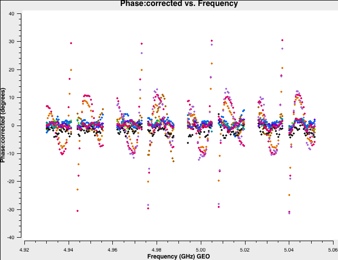
You can see that the phases have now lined up and the slopes which we saw before have mostly disappeared. We shall refine this calibration in Part 2.
6. Bandpass calibration
As you may have noticed before, when we flagged the edge channels the amplitude versus frequency of your data have a distinctive shape. This is due to the differing sensitivity of the telescope receivers versus frequency. Let's take another look at this in plotms:
## In CASA
default(plotms)
vis='n14c3.ms'
xaxis='frequency'
yaxis='amplitude'
ydatacolumn='corrected'
antenna="EF"
correlation='LL,RR'
coloraxis='baseline'
timerange='13:53:20.0~13:54:20.0'
avgtime='60'
plotms()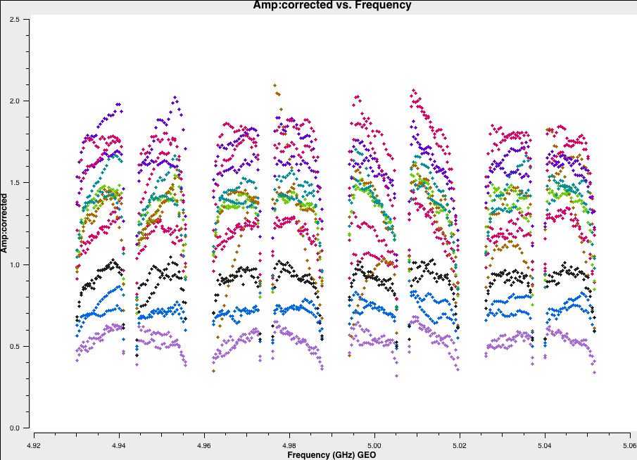
bandpass to correct this which calculates a complex gain (amplitude and phase) that corrects for the sensitivity differences. With phases, rates and delays all removed this is the only calibration issue remaining (mostly!). Again, this is an instrumental effect so we would not expect this to change with time. We can use our instrumental delay calibrator again for this. We know from instrumental delay calibration that there is enough S/N per spw. However, in order to follow the exact shape of the bandpass we now need to get enough S/N per channel! We can do this by combining all of the scans together (valid as bandpass response shouldn't change in time!):
# In CASA
default(bandpass)
vis='n14c3.ms'
caltable='n14c3.bpass'
field='1848+283'
gaintable=["n14c3.gcal", "n14c3.tsys", "n14c3.sbd", "n14c3.mbd"]
interp=['nearest','nearest,nearest','nearest','linear']
solnorm=True
solint='inf'
refant='EF'
bandtype='B'
spwmap=[[],[],[], 8*[0]]
parang=True

bandpass()
The bandpass correction should follow the shape of the amplitude response we saw earlier. Note that we set the solnorm parameter which means the calibration solutions are normalised to unity and so the total amplitudes of the data are preserved. In this case, we want to do this because our flux density scaling are done a priori and this needs to be preserved.
Let's plot the bandpass corrections, starting with the amplitude corrections (it's up to you to figure out the commands yourself!):
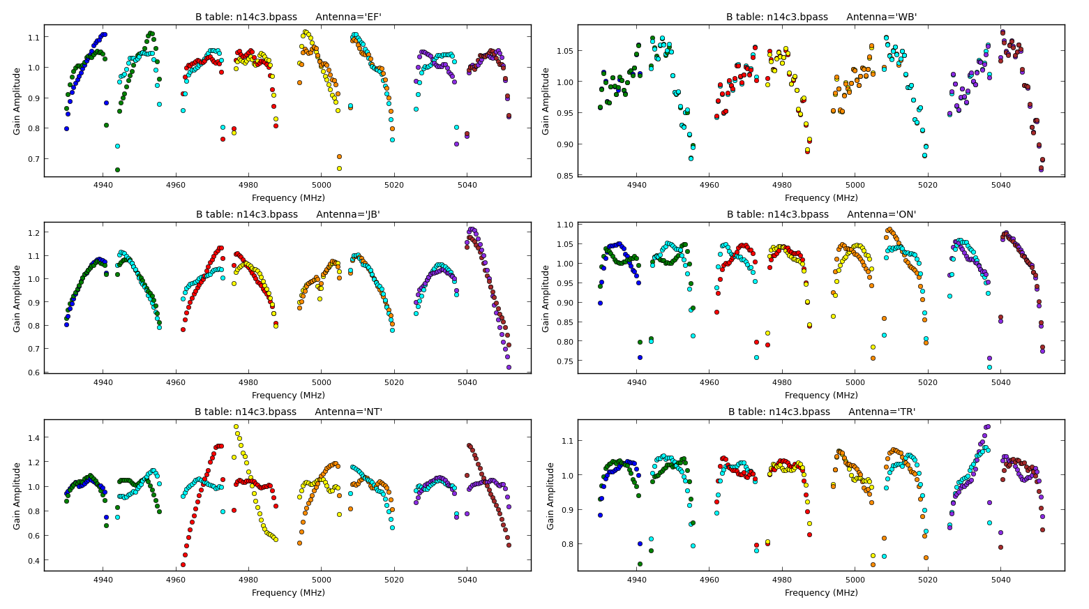
Note that, when CASA calibration tables are applied, the solution tables are divided into the visibilities which is in contrast to AIPS where solutions are multiplied into the visibilities. This means that the amplitude solutions shown here should roughly follow the visibilities as shown earlier. Let's plot the phases too. These should follow the wiggles we saw within each spectral window.
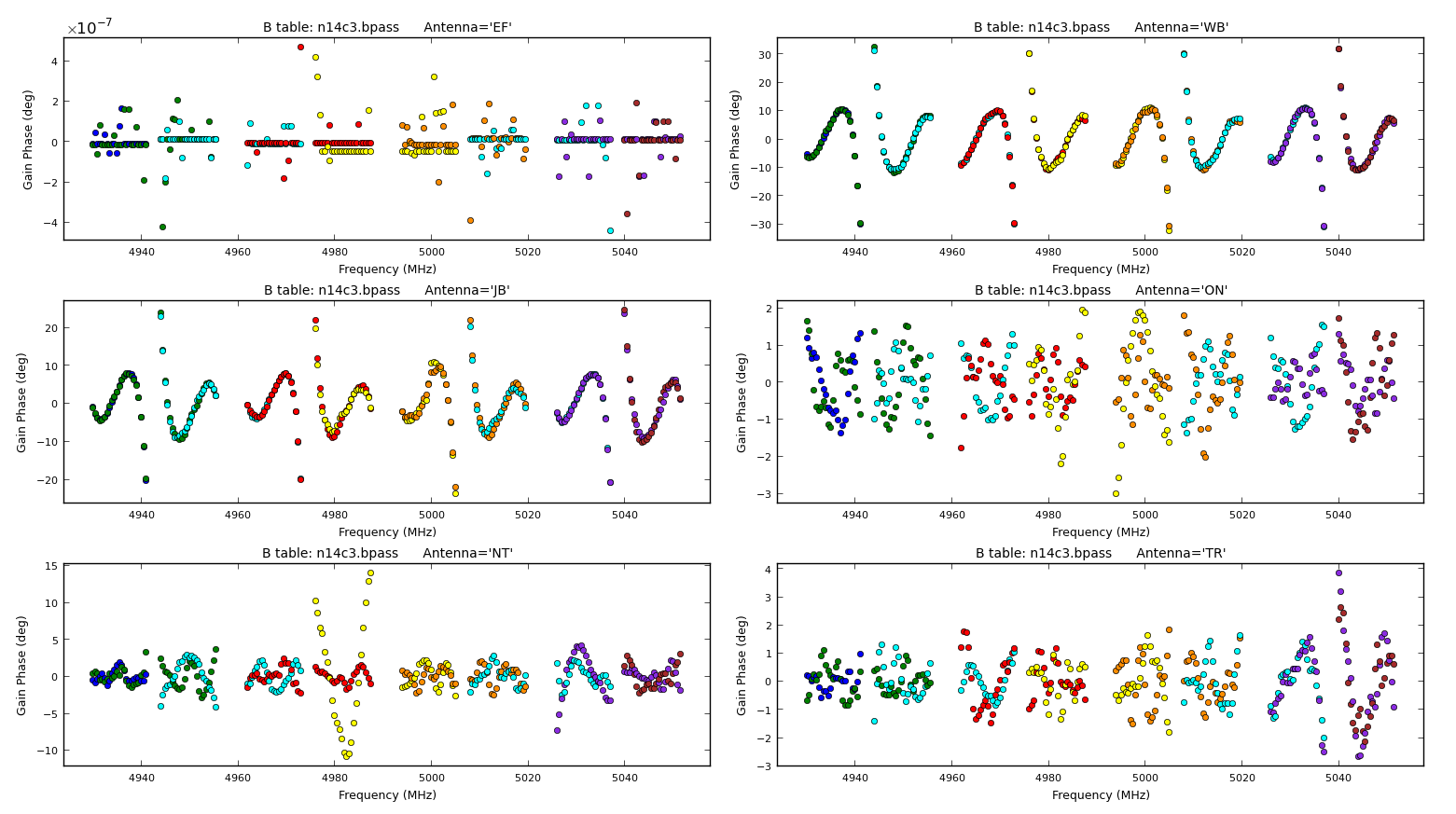
Note here that the Effelsberg telescope is our reference antenna but the phases look noisy. However, if you check the yaxis scale, you will see that these variations are of the order $10^{-7}\,\mathrm{deg}$. These are mostly computational floating point errors which are not significant at all!
These solutions look good, so we should apply this table to the data using applycal
## In CASA
default(applycal)
vis="n14c3.ms"
field=""
gaintable=["n14c3.gcal", "n14c3.tsys", "n14c3.sbd", "n14c3.mbd","n14c3.bpass"]
interp=['nearest','nearest,nearest','nearest','linear','linear,linear']
spwmap=[[], [], [], 8*[0],[]]
parang=True

applycal()
Let's have a look at what this has done to the visibilities of 1848+283. Firstly the amplitudes:
## In CASA
default(plotms)
vis='n14c3.ms'
xaxis='frequency'
yaxis='phase'
ydatacolumn='corrected'
antenna="EF"
correlation='ll'
coloraxis='baseline'
field='1848+283'
plotms()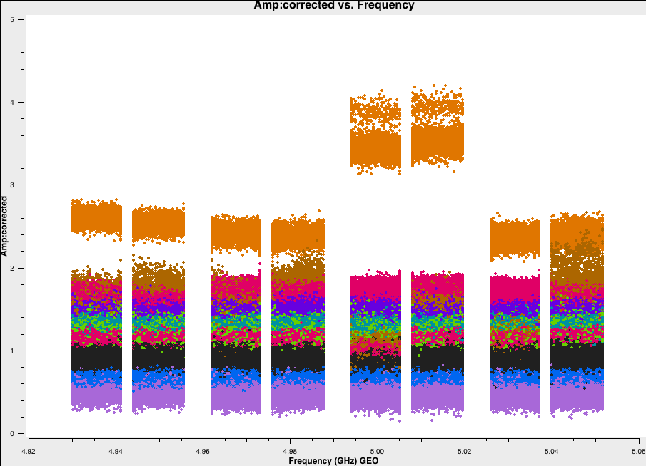
We can see that the amplitudes are scaled correctly and the bandpass shape has gone. The plot is colored by baseline and the differences in amplitudes is either due to ampltiude errors or differing flux on different baselines due to structure of the phase calibrator. If this is a true point source we would expect that the flux on all baselines is the same. We will correct these amplitudes later using self-calibration. Let's look at the phases too:
Here the phases are mostly near zero apart from one baseline which seems erroneous. We will try to fix this a little later. For now this is ok, and we can proceed to split out these data into the two phase-reference target pairs for parts 2 and 3!
6. Split out phase-ref - target pairs
The final part that we need to do is to split out the pairs of target and phase reference sources. Not only is this the necessary preparation for parts 2 and 3 of this workshop, it is also good to keep some backup copies in case future data gets corrupted or deleted. We use the task split to do this and it is straight forward to use:
## In CASA
default(split)
vis='n14c3.ms'
outputvis='J1640+3946_3C345.ms'
field='J1640+3946,3C345'
datacolumn='corrected'
split()
## In CASA
default(split)
vis='n14c3.ms'
outputvis='1848+283_J1849+3024.ms'
field='1848+283,J1849+3024'
datacolumn='corrected'
split()This completes part 1 of the tutorial. You should have been introduced to amplitude calibration, inspection and flagging of data, fringe fitting and bandpass calibration. In the following two parts we will investigate phase referencing further along with imaging and the self-calibration technique. If you have any further questions ask the DARA trainer or continue to part 2:
Part 2: Calibration & imaging of J1849+3024