 |
|
|
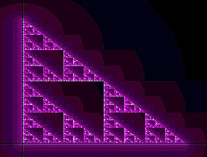
Einstein originally introduced the Cosmological Principle, the idea that the universe is homogeneous and isotropic on the large scale, mainly as an excuse to allow him to apply his new theory of gravity to the Universe as a whole, and get some answer, however unrealistic. Since then, the Cosmological Principle has often been criticised. It is perfectly possible to imagine a universe which contains structure upon structure, so that averaged over any scale, there is always something complicated going on. This idea of a hierarchical universe has been popular at least since the 17th Century.2.7In modern terms such a universe is said to show fractal structure (e.g. Fig. 2.16).
Clearly, on small scales the Universe is neither isotropic nor homogeneous, as we can tell from our own existence. Hubble claimed in the 1930s that galaxies were smoothly scattered through space, when averaged on scales larger than the size of the great clusters of galaxies (a few Megaparsecs, in modern terms). Since that time the "official" position has always been that Einstein's guess was correct: there is a scale on which the Universe becomes smooth. But there have always been mavericks arguing for a more hierarchical view.
The rough isotropy observed by Hubble can disguise quite large inhomogeneities because of averaging along the line of sight, but this can be disentangled if we map the 3-D structure of the local Universe by measuring the redshifts of galaxies.
In the 1950s Gerard de Vaucouleurs argued that galaxies within about 30 Mpc of our own Local Group were concentrated roughly in a plane, which he christened the Supergalaxy; the reality of this structure was disputed until the 1970s. Unlike a true galaxy, the Supergalaxy is not bound together by gravity: the various groups and clusters in it are moving apart according to Hubble's Law.
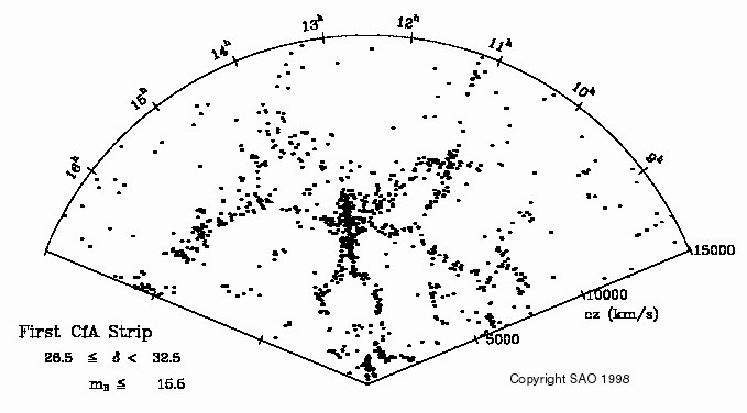
Later it was found that large `sheets' of galaxies like the Supergalaxy are a typical feature of the distribution of galaxies; in between them lie large voids where no galaxies are found. As surveys pushed further out in redshift, theorists predicted that they would soon reach the scale of homogeneity. Instead, during the 1980s each new survey found structures crossing the whole volume. A particularly striking example was the `stick man' distribution found in the CfA2 redshift survey, lead by Margaret Geller and John Huchra (Fig. 2.17). In the centre of this map, the major galaxy cluster in Coma appears as a finger pointing towards the observer: notice that it lies at the intersection of several filaments (which are actually slices through sheets). This pattern of voids surrounded by filaments and sheets, with clusters at their intersections, has become known as large-scale structure, or. more colloquially, the Cosmic Web.
 |
The 2dF instrument is making a second survey, going far deeper into the universe, by observing quasars rather than galaxies (Fig. 2.18). On the scale of quasars, there is no obvious sign of structure, but statistical analysis shows that quasars share the low-contrast structure seen on the largest scales of the galaxy survey, and even weaker, but detectable structure, on scales of 100 Mpc. It seems as if the approach to homogeneity is gradual: larger and larger structures are present, but they represent smaller and smaller fluctuations in the cosmic density.
 |
But there is one overwhelming piece of evidence that the hierarchy of structure upon structure does not continue for ever. The CMB is a window into an early universe which was astonishingly smooth and simple. In the rest of this section we will look at the simplicity of the CMB, and the implications of that simplicity for the Universe.
Penzias and Wilson had reported that their 3.5 K signal was isotropic across
the sky to `within the limits of measurement'.
According to the big bang theory, the CMB should
not be entirely isotropic. To start with, the Sun is orbiting the centre
of our Galaxy at about 220 km s-1, the Galaxy was expected to
have a small motion through the Local Group of galaxies, and by the late
1970s it was realised that the Local Group should have a motion relative
to the ideal Hubble expansion caused by the gravitational pull of more
distant matter, in particular the nearest cluster of galaxies, some
15-20 Mpc away in the direction of the constellation Virgo.
The net motion of the Sun
relative to the uniform expansion should produce a blueshift of the
CMB ahead of us and a redshift astern. Recall that the effect of a redshift
on a black body is just a change in temperature by a factor of (1 + z).
Write the average temperature as T and the maximum temperature change
as ![]() T, we expect
T, we expect
 = 1 + z,
This dipole signal was sought as soon as the CMB was discovered,
and detected in the mid 1970s. At the time, the Local Group motion was
expected to be in the direction of the Virgo cluster, but the CMB dipole
shows that the motion is about 45o away from Virgo,
and is surprisingly fast:
![]() 600 km s-1.
It was soon realised that the gravitational effect of matter
at large distances had been underestimated; mass concentrations far beyond
the Virgo cluster were affecting the motion of the Local Group.
600 km s-1.
It was soon realised that the gravitational effect of matter
at large distances had been underestimated; mass concentrations far beyond
the Virgo cluster were affecting the motion of the Local Group.
It stands to reason that the nearest structures should have the biggest effect on the motion of the Local Group. But in fact the quasi-fractal large-scale structure means that as one travels further and further away, one encounters larger and larger superclusters of galaxies, and their very large masses offset the effect of their larger distance. This started a quest to find the `convergence depth', in other words, how far away do we have to go to find all the mass concentrations that account for the dipole? To do this, we need a census of all the matter surrounding us, not just a typical slice through the universe as in Fig. 1.14. This is hard to do because quite a lot of the sky is obscured by dust in the plane of our own Galaxy. The best solution to date is to use the survey at far infrared wavelengths made by the IRAS satellite to find galaxies, as infrared radiation suffers little absorption by dust. A massive effort was therefore made to measure redshifts for all the galaxies in the IRAS Point Source Catalogue, yielding the PSCz Survey, which covers 84% of the sky (Fig. 2.19). Galactic obscuration, which prevents optical follow-up, accounts for most of the missing sky; unfortunately this includes much of the `Great Attractor' supercluster which gives an important contribution to our overall motion.
|
It seems the PSCz survey, reaching to about 250 Mpc, just about reaches
the convergence depth: its predicted dipole
is within 13o of the CMB dipole, and this difference
could be caused by the
remaining uncertainty from the unobserved region behind the Galactic plane.
While the space distribution of galaxies fixes the direction, the amplitude
of the dipole depends on ![]() ; this is a special case of the attempt
to weigh the Universe by fitting peculiar velocities, as discussed in
Section 1.4.3. The CMB dipole method is not accurate: values in the
range
0.3 <
; this is a special case of the attempt
to weigh the Universe by fitting peculiar velocities, as discussed in
Section 1.4.3. The CMB dipole method is not accurate: values in the
range
0.3 < ![]() < 1 have been deduced by various techniques, so this
is at least consistent with the favoured value of
< 1 have been deduced by various techniques, so this
is at least consistent with the favoured value of
![]()
![]() 0.35.
0.35.
It is theoretically possible that as well as the dipole due to the Earth's motion, the CMB has a primordial dipole anisotropy, the imprint of some huge gradient on much larger scales than our present horizon. Unfortunately the combination of two dipole signals is identical to another dipole in an intermediate direction, so this possibility cannot be directly checked. But most such cosmological dipoles would be accompanied by more complicated anisotropy of similar amplitude, whereas by around 1980 observations showed that, apart from the dipole, the CMB was smooth to better than 1 part in 104.
This was unexpected: small-scale fluctuations in the CMB should be present because the early universe must have contained irregularities that later grew into the large scale structure and the galaxies. In the 1970s, fluctuations were expected at a level of a few parts in 104, and the new limits on the CMB ruled this out. This turned out to be one of several strong pieces of evidence in favour of cosmological models including Cold Dark Matter, as these predict much smaller fluctuations.
Fluctuations in the CMB on scales smaller than the dipole were at last discovered by the Differential Microwave Radiometer (DMR) instrument on COBE. The DMR consisted of three units, one each operating at 31.5, 53, and 90 GHz. A block diagram of a single unit is shown in Fig. 2.20. As in many experiments designed to look for anisotropy in the CMB, each unit observed in two directions simultaneously. In the DMR this was simply achieved by rapidly switching between two identical microwave horn antennas, pointing 60o apart. All the horns had a 7o beam width. Each DMR unit contained two independent channels. At 53 and 90 GHz each channel had its own pair of horns, so that each horn spent half its time disconnected. At 31 GHz the two channels swapped between the same pair of horns in antiphase.
The rapid switching between the horns (at 100 Hz) was matched by a
synchronous demodulator which changed the sign of the signal when data
was being taken from horn number 2. After averaging, the output is then
proportional to the difference between the sky temperatures of the two
horns, T1 - T2. The rationale for this arrangement is similar
to Dicke switching against a cold load: since the net signal is very
small, small errors in the amplifier gain cannot masquerade as changes
of temperature on the sky. That is, let the output be gT, where g is
the gain and T is the system temperature (mainly produced by noise in
the amplifiers, in fact, not by the sky temperature).
If there is a gain error ![]() g,
with no switching the signal changes by
g,
with no switching the signal changes by
![]() gT, but with switching,
only by
gT, but with switching,
only by
![]() g(T1 - T2). Since the amplifier is the same, the
amplifier noise cancels precisely, as does most of the 2.7 K from the sky.
Most of T1 - T2 is an offset produced by small mismatches in the
electronics before the switch, but this is nearly constant in time.
Fluctuations in the
output are, instantaneously, dominated by noise, but also contain the
true, tiny, difference between the sky temperature between the horns.
g(T1 - T2). Since the amplifier is the same, the
amplifier noise cancels precisely, as does most of the 2.7 K from the sky.
Most of T1 - T2 is an offset produced by small mismatches in the
electronics before the switch, but this is nearly constant in time.
Fluctuations in the
output are, instantaneously, dominated by noise, but also contain the
true, tiny, difference between the sky temperature between the horns.
The DMR units were mounted on the outside of the COBE dewar as shown in Fig. 2.9; unlike most modern CMB receivers they were operated `warm' at 140-300 K. This was normal at the time COBE was first designed in the mid 1970s (receivers then were too insensitive to benefit from cooling). At the time of COBE's launch in 1989 it seemed archaic, but the cost of adding cooling for the DMR would have been enormous. A benefit from this design decision was that the DMR was unaffected when the liquid helium in the dewar ran out, and it was eventually operated for four years. This continuous operation in a weather-free environment more than made up for the relatively high noise in the receivers!
As the horns did not point along the satellite spin axis, each one swept around a small circle on the sky every 75 seconds; the centre of these circles followed the spin axis around the sky every satellite orbit of 103 minutes. Finally, as we saw when discussing FIRAS, the orbit precessed around the Earth once per year. The beams therefore swept out a complicated `spirograph' pattern on the sky, so that each 6 months every direction was observed many times by each horn.
The DMR data can be converted back into a map of the sky as follows. The sky is notionally divided up into a large number of cells or pixels. At any given time, horn 1 will be looking at one pixel and horn 2 at another. After dividing through by the gain, the DMR signal at time t is then
In the summer of 1992, after analysing just the first year of DMR data, the COBE team announced that they had discovered fluctuations in the CMB, causing a sensation. In the scientific community a major point of discussion was that the signal-to-noise ratio of the claimed detection was less than one --in other words, the typical amplitude of the fluctuations was smaller than the remaining noise at each pixel. As the CMB fluctuations were themselves expected to look very much like noise, it was impossible to tell if any particular peak in the maps was real, or due to noise. This caused some scepticism, but the analysis was sound. The true level of noise fluctuations could be simply measured by subtracting the maps made from the two independent channels (A and B) at each frequency. In these difference maps, the signal from the sky cancelled out, but the noise in the two channels was independent and so remained: as noise adds in quadrature, the rms on the difference map is given by
A more difficult problem was to show that this signal was not due to emission from our Galaxy, as the Galaxy clearly dominates the DMR maps. The COBE team had two arguments: first, they showed that the fluctuations did not decrease with distance from the Galactic plane, after excluding the belt up to ±20o from the plane. Second, by comparing the amplitude of the fluctuations at the three frequencies they showed that they had roughly constant brightness temperature, in other words, a black-body spectrum. In contrast, the brightness temperature of the Galaxy falls sharply with frequency in this range.
The final results from the most sensitive DMR unit, at 53 GHz, are shown in Fig. 2.21. With 4 years of integration, and some smoothing to give 10o effective resolution, the signal-to-noise per pixel on the CMB fluctuations is now just over 2:1; the pattern is still strongly affected by random noise, but the brightest peaks are probably real.
 |
The final COBE dipole gives an extremely accurate value for the velocity of the Sun relative to the local co-moving frame. But for cosmological purposes, we would rather know the motion of the Local Group, and unfortunately COBE did not help much with this because most of the uncertainty was already due to our inaccurate knowledge of the motion of the Sun relative to the Local Group (mainly due to its orbit around the centre of the Milky Way).
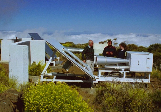
2.5.1.3 The Tenerife ExperimentsA year and a half after the first DMR result, the fluctuations were confirmed by the first significant detection of individual peaks and troughs. This was done with an experiment sited on Mt Teide on the island of Tenerife, jointly run by Jodrell Bank, the Mullard Radio Astronomy Observatory (MRAO) at Cambridge, and the Instituto de Astrofisica de Canarias (IAC). The instrument is shown in Fig. 2.22
Like COBE, the experiment measured the difference in T between two points on the sky. But ground-based experiments, even on high mountains like Teide, have to contend with emission from the atmosphere, which varies greatly across the sky. Therefore the two directions are only 8.1o apart; on this scale, the atmosphere is fairly constant. To further eliminate atmospheric fluctuations, the pointing direction is switched on a 16 second cycle by tilting a flat mirror (technically `chopping'), giving the sky response shown in Fig 2.23. The chopping mirror directs the beams nearly vertically (i.e. towards the zenith), and a circle on the sky at fixed declination is observed as it transits through the telescope beam due to the Earth's rotation. Despite these precautions a significant amount of data had to be discarded due to atmospheric emission; data was also discarded when the Sun or Moon were within 50o of the zenith, because even so far from the pointing direction they produced a significant contaminating signal.
The collaboration operated beam-switch instruments at 10, 15 and 33 GHz,
After accumulating data for several years, a clear detection was made at
15 and 33 GHz, showing consistent peaks and dips at the two frequencies,
with the same brightness temperature, i.e. a black-body spectrum.
The final results of this experiment are shown in Fig. 2.24.
Detailed comparison of these bumps with the COBE maps of the same region
showed good agreement (within the large errors of both sets of data!).
|
The COBE results set the limit to the isotropy of the Universe, at about one part in 105 on scales of 10o. When Einstein casually assumed an isotropic Universe he surely never expected his guess to be so close to the truth! A high level of isotropy is also shown by the X-ray background, at a level of around 0.2%. These X-rays are produced by numerous very distant quasars and other active galaxies, with typical redshifts of 1 < z < 3. The distribution of other objects around the sky is also more or less consistent with large-scale isotropy, but the limits are not as tight, because of smaller numbers of objects and/or larger experimental errors (e.g. Gamma-ray bursts, extragalactic radio sources).
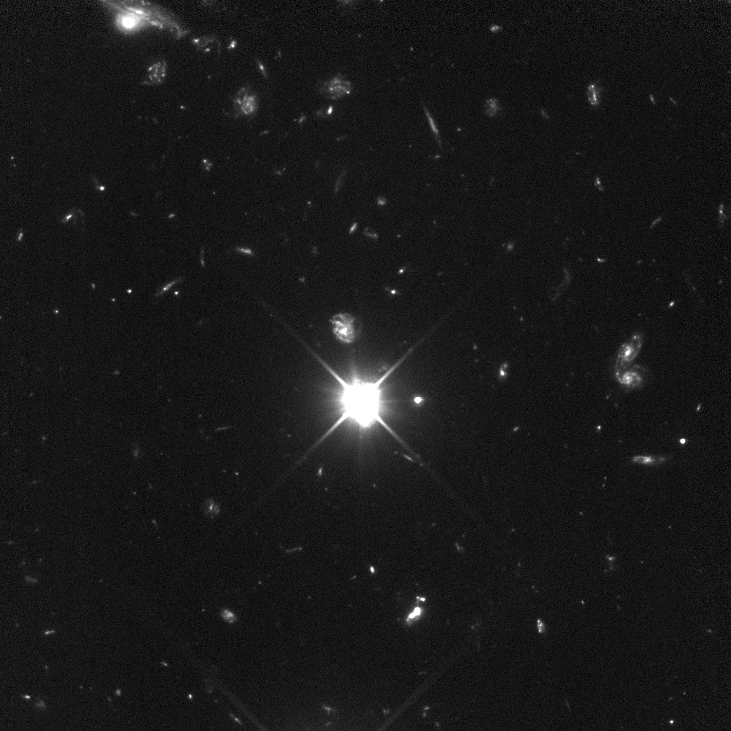
Unlike isotropy, one cannot rigorously test homogeneity, because of the
distance-time ambiguity: when we look at objects far away, we are also looking
back in time. When we see changes with distances, we assume that we are
observing evolution of the Universe over time, rather than a radial
inhomogeneity with us at the centre of the Universe. Hubble
Telescope images of galaxies out to
z ![]() 0.5
(e.g. Fig. 2.25) show that they
are very similar to ones nearby, and presumably to our own. If the
Universe was isotropic around us but inhomogeneous, observers in these
galaxies would see a very anisotropic universe. If we accept the
Copernican Principle that we are not in a special place,
the observed isotropy of the CMB and other tracers implies that
the Universe is also homogeneous on the largest scales.
0.5
(e.g. Fig. 2.25) show that they
are very similar to ones nearby, and presumably to our own. If the
Universe was isotropic around us but inhomogeneous, observers in these
galaxies would see a very anisotropic universe. If we accept the
Copernican Principle that we are not in a special place,
the observed isotropy of the CMB and other tracers implies that
the Universe is also homogeneous on the largest scales.
 |
The large-scale structure of the Cosmic Web should be a lot more stable: the pattern can change because of peculiar motions of galaxies, but the structures is so large that little change would be noticed over many billions of years. Therefore one way to look for compact topologies is to search for a repeating pattern in deep redshift surveys; this approach is known as Cosmic crystallography. Despite a couple of false alarms no such pattern has yet been seen.
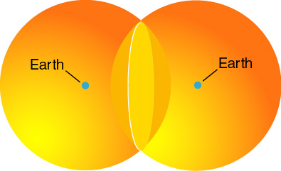
A second approach uses the CMB. To see how it works, take the view of compact topology that we appear to be in one cell of a repeating pattern. As we have seen, the sphere of last scattering surrounds us, at a distance a fraction shorter than the particle horizon. But our images appear in every other cell, and surrounding each is its own sphere of last scattering. If the repeat size is smaller than the particle horizon, these spheres will intersect; the intersection will be a small circle for any two spheres, see Fig. 2.26. Label the spheres A and B: an observer in sphere B will see the overlap with sphere A on his left, while an observer in A will see the overlap with B on his right. But A and B are the same person! So the overlap circle is seen on both sides.
Roughly speaking, the fluctuations in the CMB detected by COBE and later experiments reflect small fluctuations in the density of the universe on the sphere of last scattering. Seen from the other side, the pattern would look the same. But this is exactly what happens in a compact space: the fluctuations along the circle of intersection will be the same from each side, and so there will be two small circles on opposite sides of the sky along which the pattern of peaks and troughs will be identical. In fact in most cases there will be many such pairs of circles. To clearly detect this effect, we need maps of the CMB fluctuations covering most of the sky, and with much higher resolution than COBE. We need the resolution so that there are many peaks around each circle, to make the chance of accidental coincidence negligible. The MAP spacecraft is currently making such a survey; detection of such a compact topology would be one of the most exciting results it could produce. This mission will be described in Section 2.6.5.
Attitudes to the Cosmological Principle have fluctuated curiously through the century. To Einstein in 1917, it was a radical assumption, to be tested against observation. To E. A. Milne, in the 1930s, it was a logically necessary foundation for the whole of physics. To many astronomers since then, it has been an inference from the apparent isotropy of the Universe, which became increasingly clear over the course of the 20th century. But when the extreme isotropy of the microwave background was discovered, the Cosmological Principle began to be seen as a problem: how did the Universe become so isotropic and, presumably, homogeneous?
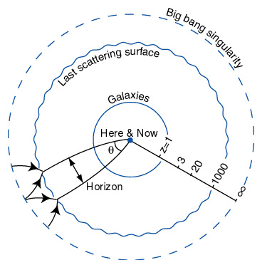
At first sight there is no problem: at the Big Bang, all points were on top of each other so it hardly seems surprising that they all started with the same temperature. But in fact, the are not at exactly the same temperature, as the COBE DMR discovered. This shows that it is not correct to say that all points were at the same place in the Big Bang: more correctly, the separation between any two points was infinitesimal -- and this in turn is a short-hand for saying that they get closer and closer together without limit if we imagine time running backwards towards the initial instant. We have already met the concept of a particle horizon (Section 1.3.4) which provides the correct way to analyse this limiting process. We saw there that a universe dominated by matter and/or radiation has a finite particle horizon which expands with time. Only parts of the Universe within each other's horizon can have communicated at any given time. The horizon length at last scattering, the "surface" of the CMB, corresponds to an angular scale of about 1o. That is, an object at the time of last scattering with a size equal to the particle horizon at that time would subtend about a degree as seen from here and now (see Fig. 2.27).
This is the Horizon Problem: how could the whole visible universe "know" to have the same temperature at the time of last scattering, when messages could not have crossed it to allow this synchronization?
There is another way of looking at this. We saw in Section 2.3.1 that, in the early universe, the temperature is set by the time since the Big Bang. So you might say that the horizon problem is the surprising(?) fact that the Big Bang happened everywhere in the Universe at (almost) the same time. Indeed, one of the several equivalent ways of describing the very small "ripples" in the temperature of the CMB is to say that there was some variation in start time from place to place!2.8
A second problem with the conventional Big Bang model is
the so-called Flatness Problem:
why is the Universe so close to Euclidean (flat) geometry? In the
next section we will see that the CMB seems to show that the Universe
is exceedingly flat. But for the moment let's ignore that. Long
ago it was obvious that there were at least some baryons in the
universe; even early counts came up with
![]()
![]() 0.01.
Recalling that in a flat universe
0.01.
Recalling that in a flat universe
![]() = 1, if we just had the minimal
number of baryons and nothing else,
= 1, if we just had the minimal
number of baryons and nothing else,
![]() = 0.01 and the universe
would seem to be quite (negatively) curved.
But extrapolating back into the past,
= 0.01 and the universe
would seem to be quite (negatively) curved.
But extrapolating back into the past,
![]() (t) rapidly rises towards one; as shown by Applet 1.12,
all Friedman models containing any matter start from
(t) rapidly rises towards one; as shown by Applet 1.12,
all Friedman models containing any matter start from
![]() = 1 (the
same applies if we include radiation). To emphasise the point, proponents
of inflation like to quote the value of
= 1 (the
same applies if we include radiation). To emphasise the point, proponents
of inflation like to quote the value of ![]() at, say t = 10-5 seconds,
which is 0.999999999999999999999999 etc. But this is a silly game as you
can get as many 9s as you like by picking an early enough time. Of course
we have no direct evidence that
at, say t = 10-5 seconds,
which is 0.999999999999999999999999 etc. But this is a silly game as you
can get as many 9s as you like by picking an early enough time. Of course
we have no direct evidence that ![]() was ever this close to one;
everything depends on the Friedman Equation. Why are we using the Friedman
Equation? Because the Universe seems to be homogeneous and isotropic. But
that is just the horizon problem, not a separate problem at all!
was ever this close to one;
everything depends on the Friedman Equation. Why are we using the Friedman
Equation? Because the Universe seems to be homogeneous and isotropic. But
that is just the horizon problem, not a separate problem at all!
There is another objection to the Flatness problem: the idea dates from the time when the Cosmological constant was out of fashion, and it was assumed that being spatially flat was to be balanced between an ever-expanding universe and one that re-collapses. But as Applet 1.12 shows, the actual divide between these options is more to do with the sign (and size) of the Cosmological constant than to do with spatial flatness. Even so, there is a real problem buried in the confusion. At some time, the universe either recollapses, or it starts to expand exponentially (it used to be assumed that this is the time when it departs substantially from flatness, but with a cosmological constant it may remain close to flat at all times). This gives an expansion timescale. Now the nub of the problem is, how come the expansion timescale is so long? This is better named the Oldness Problem.
It is reasonable to ask, long compared to what? Particle physicists would like us to believe that the natural timescale for the Universe is the Planck time, 10-43 seconds. On this basis we have a very severe oldness problem indeed! Obviously, the particle physicists are wrong; in fact we have no idea what sets the "natural" expansion timescale: in effect it is a fundamental constant of nature (on the basis that any value we can predict from more basic physics is not fundamental). Now, we can come up with many other timescales for important processes, for instance the times for baryons, nuclei, atoms, stars and galaxies to form. These timescales differ from each other by many orders of magnitude.
 What are the timescales for the formations of baryons, nuclei and atoms?
Review Section 2.3 to remind yourself. (We will come to the formation
of stars and galaxies in the last section of this module).
What are the timescales for the formations of baryons, nuclei and atoms?
Review Section 2.3 to remind yourself. (We will come to the formation
of stars and galaxies in the last section of this module).
|
For reference, the first stars form several
hundred million years after the big bang, at t ![]() 1016 seconds, while clusters formed
around z = 1, about 5 billion years after the Big Bang, t
1016 seconds, while clusters formed
around z = 1, about 5 billion years after the Big Bang, t ![]() 1.5×10¹⁷
seconds.
1.5×10¹⁷
seconds.
Each timescale is set by its own particular combination of the fundamental constants, and if the constants had had different values, these events would have happened in a different order. Should we now be surprised that the the expansion timescale is longer than all of these? It is lucky for us that it is, because we would not be around if the universe had recollapsed before baryons (or galaxies) had formed; and exponential expansion is also deadly: if this had started before, say, atoms were formed, protons and electrons would have become too separated to meet up, and the development of the universe would have been cut short. Certainly we should suspect some conspiracy if the expansion timescale was the longest of all, but in fact there are physical timescales which are far, far longer than the present age of the Universe: the time for proton decay, for instance, or for evaporation of black holes through Hawking radiation. So in the end the oldness problem boils down to the fact that the expansion timescale is the longest of a dozen or so crucial timescales for an "interesting" universe, a priori, a probability of about 1 in 12, which to a scientist is surprising enough to merit some serious thought, but not a publication!
There is one last problem with the Big Bang, which is the opposite of the Horizon Problem: given that there is obviously an effective (although unknown) way of making the universe smooth, how come there is any structure in the universe? This is the Structure Problem. We will see in Section 2.6.1 that stars and galaxies are formed by gravitational collapse from small fluctuations in the density of the early universe. We will be able to be quite definite about how "small" these fluctuations were, and it turns out that they are far too big to have arisen purely by the random motion of particles. So we can re-phrase the structure problem as: where did the density fluctuations that lead to stars and galaxies come from? We will see that these same fluctuations are responsible for the small-scale anisotropy of the CMB discovered by COBE.
The various problems with the standard Big Bang model listed in the previous section are solved in the inflationary universe scenario, and it is often justified on this basis. However, other solutions have been suggested for the most concrete of the problems, the formation of structure, and in fact a much better motivation to look at inflation is that its specific predictions about the fluctuations in the universe match observations remarkably well. This has convinced many previously skeptical cosmologists that something like inflation may really have happened.
Inflation theory begins with particle physicist Alan Guth of MIT. In the late 1970s, Guth was working on a theory designed to supercede the present `standard model' of particle physics, a so-called Grand Unified Theory that tied together the Strong, Weak, and Electromagnetic forces of nature. The theory was promising, but Guth realised it had a major drawback: it predicted the existence of large numbers of magnetic monopoles, the magnetic equivalent of electrons, carrying a single magnetic `charge', that is, an isolated North or South pole. Unfortunately for Guth, physicists had been searching for magnetic monopoles (which appear in many different theories) for most of the century, with no success. To be consistent with this result, Guth needed to drastically reduce the density of monopoles predicted by his theory. One day he hit on a simple way to do it. According to quantum theory, particles can be considered as waves in an underlying field. These waves are quantised, that is their amplitude can only have discrete values: the idea is that if the wave amplitude goes up by one unit, we say we have added one more particle. The simplest kind of field is called a scalar field, and it has a well-known peculiarity: even with no particles, the oscillations have a finite amplitude, and an associated energy, the so-called zero-point energy. Since the zero-point energy is always there, and unchanging, it has no effect on the kind of things most particle physicists were studying, so nobody paid much attention to it. But Guth realised that such a zero-point energy had all the properties of the cosmological constant: a fixed energy density, the same at all points in the universe, that was unaffected by expansion.
The energy density of a plausible quantum field would be enormous, giving an exponential expansion timescale of 10-35 seconds or less (for exponential expansion the timescale is the Hubble time, tH = 1/H). But this was just what Guth needed. His irritating monopoles would be produced by GUT interactions in the very early universe, but as the universe expanded the energy density of radiation fell, and at 10-35 seconds after the Big Bang the zero-point energy of his hypothetical quantum field would dominate, and exponential expansion would begin. By, say 10-33 seconds after the big bang ( t = 100tH), the universe would have expanded by a factor of eHt = e100 which is a very large number. The monopoles would be spread so far apart by now that the chance would be remote that there was even one lurking in the whole observable universe! Of course, any other pre-existing particles would have been equally diluted. This period of early exponential expansion Guth called `inflation'.
As we have seen (e.g. from Applet 1.12), any universe with a
positive cosmological constant quickly moves to the de Sitter solution,
which is spatially flat. In fact in 100 expansion timescales,
|![]() - 1|
is reduced by a factor of
e-200 = 10-87, so the flatness is very
exact! The rapid expansion quenches the temperature of the
primordial heat bath; by the same factor, in fact, so we can take the
temperature as essentially zero.
- 1|
is reduced by a factor of
e-200 = 10-87, so the flatness is very
exact! The rapid expansion quenches the temperature of the
primordial heat bath; by the same factor, in fact, so we can take the
temperature as essentially zero.
Now Guth's only problem was to stop inflation carrying on for ever.
The basic idea is that the scalar field
responsible for inflation somehow converts its energy into particles of
ordinary matter. The universe goes from T = 0 with a large energy in the
scalar field to one where the energy density
![]() c2 is equal to
the previous scalar field energy density: this implies a very high
temperature, hence the process is called reheating.
c2 is equal to
the previous scalar field energy density: this implies a very high
temperature, hence the process is called reheating.
|
The temperature immediately after reheating should be almost
the same as the temperature just before inflation started. Why?
|
Ironically, the monopole problem that originally motivated inflation has now evaporated. The GUT theory that Guth was working on has been conclusively disproved on other grounds, and although other GUT theories are still possible, most of them do not predict large numbers of monopoles. But inflation does solve the horizon and flatness/oldness problems. Let's see how.
After reheating, the Universe continues to expand just as in the normal
hot Big Bang, but it is now almost perfectly flat.
To see whether this is enough to solve the oldness problem, let's simplify
by assuming that the universe stays radiation-dominated until now, at
t ![]() 1017 seconds after the Big Bang. Then we have
R
1017 seconds after the Big Bang. Then we have
R ![]()
![]() ,
so between 10-33 and 1017 s, the universe expands by a factor
of
,
so between 10-33 and 1017 s, the universe expands by a factor
of
![]() = 10(17 + 33)/2 = 1025. In a
radiation-dominated universe,
|
= 10(17 + 33)/2 = 1025. In a
radiation-dominated universe,
|![]() - 1| is proportional to the square
of the expansion factor, so it increases from around 10-87 right after
inflation to
1050 - 87 = 10-33, which is still very small!
Of course, I pulled
the value of 100 expansion timescales out of a hat, but it does
show how easily inflation can make a flat universe.
- 1| is proportional to the square
of the expansion factor, so it increases from around 10-87 right after
inflation to
1050 - 87 = 10-33, which is still very small!
Of course, I pulled
the value of 100 expansion timescales out of a hat, but it does
show how easily inflation can make a flat universe.
|
If there were only 50 expansion times during inflation, when would the
later evolution of the universe make it curved again?
|
Because small changes to the length of the inflation period
have a huge effect on
the subsequent size (or flatness) of the Universe, inflation tends to
either over-solve the flatness problem, making the universe very close to
flat, or it fails to solve it at all (the universe becomes curved very
long ago). So a clear prediction from inflation, given that the
Universe is observed to be at least roughly flat, is that really the Universe
is almost perfectly flat: detailed models give
|![]() - 1|
- 1| ![]() 10-5.
10-5.
Guth's solution to the horizon problem is trivial: everything is at the same temperature because, in fact, the true particle horizon at the time of last scattering was much bigger than the observable universe. Before inflation began, the presently observable universe was so small that it could very quickly and easily come into equilibrium. Our earlier calculation of the horizon size was wrong because we did not allow for the inflation period, during which the particle horizon expands exponentially. In fact the conventional calculation gives a useful "pseudo" horizon, which applies to any signal setting out from after the end of inflation (only 10-33 s after the Big Bang, so this applies to nearly all signals!).
The solution to the structure problem is not trivial at all (and is not part of Guth's original concept). Let's have a closer look at the idea of quantum fields. One of the core concepts of quantum theory is uncertainty, and one of the quantum uncertainty principles is written:
But things change when space is exponentially expanding. The quantum fluctuations are caught up by the expansion and inflated to macroscopic sizes before they have a chance to disappear. (This is closely related to Hawking radiation from a black hole, where again virtual particles and anti-particles are separated by a strong gravitational field which forces them to become real). What is fluctuating? In short, everything: density, temperature, pressure, etc. But it happens in such a way that the relation between these is preserved; so that a denser-than average region at the peak of a ripple (an over density) evolves just as the Friedman equation says, but the time is slightly out of synch with a neighboring under-density. Fluctuations in which density and temperature fluctuate together in this way are called adiabatic.
The amplitude of these fluctuations is determined by the detailed physics of the relevant quantum field, which is the inflation field. For definiteness, think of each fluctuation as a ripple with a particular wavelength and orientation. The net effect is the superposition, or mutual interference, of a whole spectrum of such waves. Experimentally, we will see that the density fluctuations have amplitudes around 2 parts in 105. A clear prediction of inflation is that, with all the ripples superimposed, the probability of having any particular density at each point is described by the classic bell curve, i.e. a normal or Gaussian distribution. To be specific, when I quote amplitudes, I'm referring to the standard deviation, defined so that 68% of points are within 1 standard deviation of the mean density.
To simulate a cosmological constant, the average energy of the inflation field must be constant. Actually, in most theories, the energy changes, but slowly enough that we can take it as constant as a rough approximation. This means that the density fluctuations produced at any time during inflation have about the same amplitude and the same chance of having any initial wavelength. But depending on the time that each ripple sprang into being, it will be inflated by a different amount: the ones that happen early will be stretched beyond the size of the visible universe, while the last will correspond to cosmologically tiny scales, say just a few metres. The superposition of fluctuations created all the way through inflation will give ripples of every wavelength, all with roughly the same initial amplitude of 2×10⁻⁵.
To summarise, the idea is that all the observed structure in the Universe started as sub-microscopic quantum fluctuations during the epoch of inflation! Furthermore, inflation predicts that the fluctuations should be adiabatic, gaussian, and have an amplitude almost independent of wavelength. These are all testable predictions.
Inflation neatly solves the horizon and oldness problems, and gives a spectacular theory for the origin of structure, but the cost is high. We have a previously unsuspected quantum field, whose detailed physics is unknown (there are many competing theories). This physics controls the times (or temperatures, if you prefer) that inflation began and ended (so we don't really know these times; the values I quoted earlier were just guesses), and also the details of the crucial reheating process. This gives many different inflation theories, all giving very similar predictions so it is hard to imagine observations which could tell which one is right.
Inflation also provides an impenetrable barrier to understanding even earlier times, because it wipes the slate absolutely clean, as we saw with the monopoles. But there is one point worth making about the universe before inflation. Guth assumed that initially the universe was expanding as per the normal Big Bang model, in other words, that it was homogeneous and isotropic before inflation. This makes no sense if inflation is supposed to produce the homogeneity of the universe, so nowadays we imaging that inflation began in a chaotic early universe, in which space-time and the quantum fields it contains fluctuated with large amplitudes on a wide range of scales. In such a universe we should not really speak of "time since the Big Bang"; in fact this chaotic stage could last a long time or even forever. Here and there in the storm, conditions become "just right" for inflation to take off, and that small part of the chaotic universe becomes the seed for a universe like ours, or perhaps more often, not like ours at all!
![\begin{picture}(6,10.7)
% put(0,0)\{ framebox(6,10.7)\{ \}\}
\put(0,0){\includegraphics*[width=6cm]{ten_beam.eps}}
\end{picture}](img188.gif)
![\begin{picture}(12,8.5)
% put(0,0)\{ framebox(12,8.5)\{ \}\}
\put(0,8.5){\includegraphics*[height=12cm,angle=-90]{cmbgal.eps}}
\end{picture}](img189.gif)