2.6 The formation of structure in the Universe

We have seen how inflation theory predicts the formation of fluctuations in the universe. In this section we will first look at how such fluctuations could grow to become galaxies and clusters of galaxies. Then we will see how, long before galaxies form, these fluctuations leave their imprint on the CMB, and we will see how CMB observations are dramatically confirming some of the key predictions of inflation. We can directly compare the fluctuations at the time of the CMB with those in the Universe today, as measured by the new large galaxy redshift surveys. Finally, we will look at the future of CMB studies, particularly the space missions MAP and Planck.

2.6.1 Gravitational Runaway

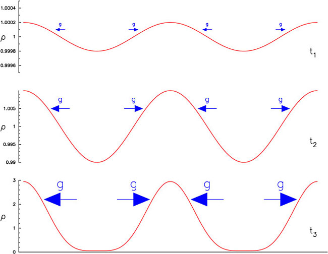
Gravity is a natural destabiliser. If there is any fluctuation in the density of the cosmic fluid, the local gravitational force points towards the nearest density peak, pulling material out of the under-dense regions towards the over-dense regions. The extra mass increases the density of the peaks, increasing the amplitude of the gravitational force, so the fluctuations amplify faster and faster. If there was no universal expansion, fluctuations would grow exponentially. At first, a pure sinusoidal ripple would maintain its form, simply growing in amplitude. Furthermore, any more complicated fluctuation can be analysed in terms of superimposed sinusoids, each of which grows independently of the others. The total fluctuation is just the sum of all the sine waves (a so-called linear superposition). But when the density variation becomes comparable to the mean density, the growth becomes non-linear, and the shape distorts: ripples of different wavelength interact and the theory becomes far more complicated. Non-linearity is inevitable for large amplitudes, because the density can't fall below zero (see Fig. 2.28).

Figure 2.28: Gravitational growth of a density fluctuation.

The growth of density fluctuations in the Universe is counteracted by

• The overall expansion of the universe, which reduces the exponential growth to at most a power law, i.e. amplitude $\propto$ t^a, where a depends on the expansion law (radiation vs. matter dominated, etc).
• The higher pressure in the density peaks, which resists their gravitational collapse.

A nice result from Newton's theory of gravity is that a blob of density $\rho$, with no internal pressure to support it, will collapse to a point in about 1/$\sqrt{G\rho}$ seconds, irrespective of the size of the blob. Qualitatively, this works because bigger blobs have stronger gravitational fields and so collapse faster. Sir James Jeans worked out what happens if we allow for pressure. Then, sound waves can travel through the blob; the sound speed is roughly c_s $\approx$ $\sqrt{P/\rho}$. This will take a time L/c_s, where L is the size of the blob. If this time is longer than the collapse time, the sound waves `tell' the interior to increase its pressure to oppose the collapse, and the blob will `bounce'. On the other hand, if the blob is too big, the collapse overtakes the sound wave and pressure does not have much effect. Applied to a ripple of a single wavelength, the same arguments show that if the ripple wavelength is smaller than the Jeans length

$$\lambda_{J}^{}$$ = c_s$$\sqrt{\pi \over G \rho }$$

then the ripple will oscillate as a standing sound wave; otherwise it will suffer runaway gravitational collapse as shown in Fig. 2.28.

After nucleosynthesis has finished, we saw in Section 2.3.4 that the stuff of the Universe consists of a photon-baryon fluid with a large (relativistic, in fact) pressure, together with Hot Dark Matter made of neutrinos and Cold Dark Matter made of WIMPs; neither of which feel pressure. Now remember that inflation predicts adiabatic fluctuations, which implies that all these components initially fluctuate together: in some regions all are over-dense, elsewhere all are below average density. Now let's follow a single ripple as the universe expands. It is conventional to describe it by its co-moving wavenumber

k = $${2 \pi \over (1+z) \lambda}$$

At any time, $\lambda$ is the physical wavelength. As the fluctuation expands with the universe, this increases with time, but the scale factor (1 + z) allows for this so that k is unaffected by expansion (which is why we call it a co-moving value).

At first the wavelength $\lambda$ will be much larger than the local Hubble radius, c/H(t), which we call the horizon. This is a rough approximation to the particle horizon, or rather, the pseudo-horizon (c.f. Section 2.5.3): the distance that a non-interacting particle can travel from the end of inflation until time t. At this time, the peaks and troughs of the ripple are out of causal contact with each other (since the end of inflation), so the only thing that happens is that the wavelength expands along with the Universe. One can ask, does the amplitude of the wave increase or decrease during this phase? The irritating answer is that it depends on the coordinate system you choose -- another manifestation of the relativity in GR!

The situation changes when the expansion of the horizon with time catches up with the wave, when c/H $\sim$ $\lambda$ = 2$\pi$/(1 + z)k. At this point, horizon entry, inflation predicts that the amplitude of all waves should be roughly the same. From now on, all coordinate systems agree. Amplitudes are very small, with fluctuations in the density of a small fraction of a percent. If the wavelength is small enough that horizon entry happens during the radiation era, gravitational instability is suppressed by the overall expansion, and the fluctuation does not grow in amplitude.^2.9 Detailed calculations show that horizon entry is in the radiation era if

(1 + z)$$\lambda$$ < $${16 { \rm Mpc} \over \Omega_m h^2}$$.

In fact, these ripples are slightly damped. This happens because the neutrinos, unaffected by pressure (or anything else) are moving in random directions at essentially the speed of light. These random motions smooth out the original density fluctuations in the neutrinos, starting with the ripples with the smallest wavelengths. The ripples in the CDM and photon-baryon fluid are at first unaffected by this.

As the universe approaches matter-radiation equality the expansion law for the universe begins to change, eventually reaching R $\propto$ t^2/3 in the matter-dominated era, as we saw in Section 1.3.3. In the absence of pressure, this allows some gravitational instability, with the amplitude of density fluctuations growing in proportion to R. This is exactly what happens to the CDM fluctuations. At this point, the smoothing of the neutrino ripples would have been important if neutrinos had dominated the matter density. Then, the small-scale ripples would have been heavily damped, and so structure on scales smaller than a few Mpc would have been very slow to form. One strong piece of evidence against very massive neutrinos (or any other form of Hot Dark Matter) is that these small ripples do not seem to be damped.

Meanwhile, fluctuations in the photon-baryon fluid that have entered the horizon oscillate as standing sound waves rather that grow, because just after matter-radiation equality the Jeans length is roughly the horizon scale, $\lambda_{J}^{}$ $\sim$ c/H (fluctuations outside the horizon are still in the ambiguous GR phase).

Given that the sound speed is c_s = c/$\sqrt{3}$ (Section 2.3.4, use the Friedman equation (with k = 0) to show that the Jeans length is

$$\lambda_{J}^{}$$ = $${\sqrt{8} \pi \over 3}$$ $${c \over H}$$.

Answer

The Jeans length is defined by

= c_s

From the Friedman equation with k = 0 we have G = 3H²/8. Inserting this and the relativistic sound speed we get

=   =  .

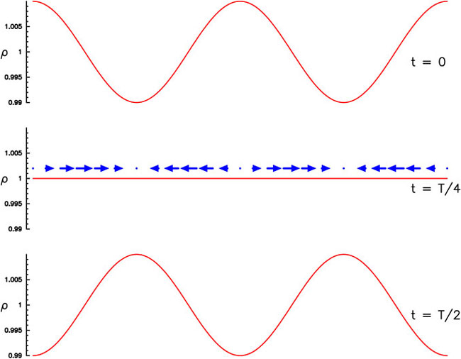
Because the start time for oscillations is set by horizon entry, all waves with a given wavelength should oscillate in phase. Recall that a standing wave (e.g. a wave on a string) goes through nulls, times when the amplitude is zero, but the motion is a maximum (Fig. 2.29). Therefore, at any given time, all ripples which have wavelengths corresponding to 1/4, 3/4, 5/4, etc periods since horizon entry should be null, while ripples with wavelengths corresponding to 1/2, 1, 3/2 etc. periods since horizon entry should have their peak amplitudes.

Figure 2.29: A standing wave at three times during its oscillation separated by a quarter of the full period.

After some time, the sound speed in the photon-baryon fluid begins to fall from the relativistic limit, as the falling photon energy density begins to approach the rest mass density of the baryons. This means the Jeans length becomes slightly smaller than the horizon (it continues to grow, but not quite as fast as the horizon), and so photon-baryon fluctuations have a brief opportunity to grow between entering the horizon and being overtaken by the Jeans length. This phase happens just before last scattering, and at that time we have relatively large amplitude fluctuations in the CDM (though still small enough to be linear), and oscillations in the photon-baryon fluid with roughly the original amplitude, except that scales close to the horizon have grown a bit. But once the free electrons bind to atoms, the photons stop interacting. The random motions of the baryons (now hydrogen and helium atoms) is very small, in other words, with the photons out of the picture, the baryon pressure and sound speed plummets, and the Jeans length becomes very small. Because the CDM makes up most of the mass, it dominates the gravitational forces, so the baryons fall into the potential wells defined by the CDM, and from this time on the CDM and baryons can be treated as a single pressureless fluid.

Notice that all fluctuations which enter the horizon during the radiation era start with the same amplitude, and start growing at the same rate at the same time, at matter-radiation equality. They therefore remain all with roughly the same amplitude. On the other hand, bigger fluctuations, that enter the horizon during the matter era, start with roughly the same amplitude (according to inflation theory), but have less time to grow, progressively less, in fact, for bigger and bigger scales, which enter at later and later times.

The primordial spectrum produced by inflation is usually taken as a power law, i.e. the power in fluctuations with wavenumber k is:

$$\cal {P}$$(k) $$\propto$$ k^{n - 1}

The index is written n - 1 rather than n for historical reasons. The value n = 1 corresponds to constant power on horizon entry for all k, which is known as a scale-invariant spectrum. Inflation predicts that the spectrum should be close to scale-invariant: n = 1 exactly would be predicted for pure exponential inflation, i.e. a constant energy density for the inflationary field. In fact the inflationary field must change towards the end of the inflationary period (otherwise it would not end) and so small departures from n = 1 are expected.

The resulting power spectrum of fluctuation amplitude is shown in Fig. 2.30. It is worth emphasising that for a given cosmological model and theory of inflation, the predicted fluctuation spectrum at this stage can be calculated as accurately as we please, (although an accurate calculation is very complicated and in practice takes a lot of computer time to do!). This is because we can treat fluctuations with each wavenumber independently.

Figure 2.30: Plot of rms amplitude of the fluctuation against wavenumber k. Notice that long wavelengths (small k) are on the left! Technically, this plot is the square root of the power spectrum. The form of this spectrum depends weakly on cosmological parameters such as $\Omega$: the red curve is for h = 0.65, $\Omega_{m}^{}$ = 1, $\Omega_{\Lambda }^{}$= 0, and n = 1 ("standard cold dark matter"); the blue curve is the same but for $\Omega_{\Lambda }^{}$ = 0.7, $\Omega_{m}^{}$ = 0.3. The overall amplitude scale is arbitrary.

Eventually, the fluctuations become so large that their growth becomes non-linear. From Fig. 2.30 the first fluctuations to reach non-linearity are the ones on small scales, a few co-moving Mpc or less. We observe galaxies at z = 6 which shows that at least some fluctuations have become non-linear before then, say at z $\approx$ 10, about a billion years after the Big Bang. As the amplitude grows $\propto$ R $\propto$ 1/(1 + z) in the linear phase, you should be able to calculate that we need fluctuations with amplitudes of around 10^-3 at last scattering. In a baryon-only universe, the fractional temperature fluctuations of the CMB would tell us the fractional density fluctuations in the matter at last scattering, which is why the isotropy of the CMB ruled out this model. As we have seen, the cold dark matter can have much larger fluctuations than the photon-baryon fluid at the time of last scattering, because they have been growing ever since the universe ceased to be completely dominated by radiation.

Once non-linearity sets in, we no longer have a superposition of individual sinusoidal ripples: the development of each ripple depends on all the others, and the physics becomes far too complicated to follow in detail. But in essence, the high-density peaks suffer run-away collapse, forming first the smallest structures (the first stars), then very soon after, galaxies. This process can only be studied by numerical experiments in computers. For some state-of-the art results, look at the VIRGO consortium web site. Even these simulations necessarily leave out many important processes: star formation, stellar winds, shock waves, magnetic fields... theoretical cosmologist Richard Bond calls this phase `gastrophysics'. It marks the border between the theoretical clarity of cosmology and the more seat-of-the-pants theory that characterises the rest of astronomy.

Fluctuations on larger scales than a few Mpc lag in their growth, and becomes non-linear significantly later. Thus, the most distant known galaxy has z = 6.56, but there are no known large clusters of galaxies with z > 1.5.

The final stage of the formation of structure happens when the matter era ends, that is, when $\Omega_{m}^{}$ falls significantly below 1. At this point, growth of structure stops; we can say that gravity freezes out, just as the weak and electromagnetic forces did in the early Universe. This is happening about now. Ripples with wavelengths longer than around 30 Mpc are still in the linear phase, and from now on will simply expand along with the universe without changing their amplitude. This is important because, to repeat, we can predict accurately in the linear regime.

2.6.2 Fluctuations in the Cosmic Microwave Background

You may be wondering why we paid such attention in the last section to the Jeans length and standing sound waves in the photon-baryon fluid, when in the end the baryons precisely follow the CDM: the more complicated physics of baryons had no lasting effect on structure formation. The answer is that the CMB gives us a cosmic CAT scan of the Universe at the moment this phase of standing sound waves ended.

We saw in Section 2.3.4 that CMB photons travel direct to us from the surface of last scattering. This sphere is special only in the sense that photons from there happen to reach us now; otherwise the surface is a typical `slice' through the Universe at the time photons decoupled. The slight fluctuations in the CMB temperature discovered by COBE are a direct view of the density fluctuations and sound waves in the photon-baryon fluid.

2.6.2.1 The Angular spectrum

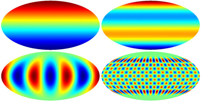
In the previous section we analysed the fluctuations in terms of sine-wave ripples, each characterised by its wave number and direction. One can make an equivalent analysis of fluctuations on a sphere in terms of patterns called spherical harmonics. Fig. 2.31 shows a few of these. Each harmonic is characterised by two integers, l and m: the multipole l corresponds roughly to k, so that a spherical harmonic with multipole l has peaks with angular size roughly $\psi$ $\sim$ $\pi$/l radians. For each multipole l there are 2l + 1 possible values of m (from - l to + l) which define the fine detail in the spherical harmonic pattern.

Figure 2.31: Some spherical harmonics, 'ripple' patterns used to analyse the temperature pattern of the CMB. At top left is a dipole, Y_{1, 0}; top right and bottom left are the octupoles Y_{3, 0} and Y_{3, 3}, and bottom right is a higher multipole, Y_{20, 12}.

Fluctuations in the CMB will have distinctly different properties depending on their scale $\lambda$ (corresponding to angular scale $\psi$ = $\lambda$ / D_A(LS) where D_A(LS) is the angular size distance to the sphere of last scattering).

Obviously there is no exact correspondence between spherical harmonics and sine waves, but use the formulae given above to estimate the co-moving wavelength (1 + z)$\lambda$ corresponding to fluctuations with multipole l. (Recall that the co-moving value is the present-day size, because the Universe has expanded by a factor (1 + z) between then and now).

Answer

We have

(1 + z) = (1 + z)D_A = R₀S_k() R₀S_k()/l

From Fig. 1.10, R₀S_k() for redshift 1000 (essentially, for our particle horizon) is about 1.5×10⁴ Mpc (for h = 0.65), i.e. 15 Gpc, so we have

(1 + z)  Mpc

For instance, the first acoustic peak (see below) has l 200, corresponding to 250 Mpc.

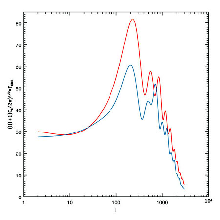
Inflation theory predicts the mean-square values C_l of the amplitudes of each spherical harmonic. These do not depend on m, and so we can estimate the observed C_l values by averaging the amplitude of all the harmonics with multipole l. A plot of l (l + 1)C_l/2$\pi$ against l is known as the angular spectrum. This apparently complicated form is picked because it corresponds roughly to ($\Delta$T)²($\psi$), where $\Delta$T($\psi$) is the rms fluctuation in temperature observed on angular scale $\psi$. A typical predicted angular spectrum is shown in Fig 2.32; we will now look at each of the key features of this spectrum.

Figure 2.32: The angular spectrum (C_l spectrum) predicted for the two models in Fig. 2.30.

2.6.2.2 The Sachs-Wolfe Effect

On the largest scales we will see ripples which are still bigger than the horizon, and so unaffected by causal processes since inflation. I mentioned that the amplitude of these fluctuations depends on the coordinate system used to describe them; but of course the observable fluctuations in temperature do not! These fluctuations are known as the Sachs-Wolfe Effect. The fractional temperature fluctuation turns out to be -1/3 times the fluctuation amplitude on horizon entry, and so $\Delta$T($\psi$) will be constant with $\psi$ if the spectrum is scale-invariant. The minus sign means that regions of overdensity correspond to cool spots and vice versa; one way to explain this is to say that photons leaving denser regions must climb out of a slightly deeper gravitational well, thereby loosing some energy. The fluctuations discovered by COBE were due to this effect.

The COBE fluctuations corresponded to $\Delta$T = 18 $\mu$K. Show that this leads to a value for the density fluctuation on horizon entry of 2×10^-5, as quoted in the previous section.

Answer

For T = 2.725 K and T = 18K, we have a fractional temperature fluctuation of T/T = 6.6×10^-6. From the Sachs-Wolf formula, this is 1/3 of the density fluctuation, which must then be

3×6.6×10^-6 = 1.98×10^-5.

close enough to 2×10^-5, given the uncertainty in the measurements of T.

2.6.2.3 Acoustic Peaks

We have seen that the critical length scale for structure at any time in the history of the Universe is the horizon at that time. Actually we can be a bit more precise: in reality, different parts of the photon-baryon fluid react to each other by exchanging sound waves, so the crucial length is the sound horizon c_st $\approx$ ct/$\sqrt{3}$, a bit shorter than the light horizon ct. On scales shorter than this we are in the regime of standing sound waves or acoustic oscillations in the photon-baryon fluid. In this regime, hot patches on the sky correspond to regions of high density, as they correspond to over-densities of photons as well as baryons, and the gravitational potential of small fluctuations is not enough to overcome this (because the fluctuations are oscillating, their Doppler shifts will also have an effect on the temperature, but this is smaller than the effect of density). As we saw in the previous section, scales just inside the (sound) horizon have had a chance to grow slightly, and should be near the peak of their oscillation; so we would expect to see enhanced fluctuations on this scale, or to put it another way, we should find a peak in the angular spectrum for l values corresponding to the sound horizon. On somewhat smaller scales, all fluctuations will be at a null, and on smaller scales still, another peak, but one that had less chance to grow because these waves entered the horizon earlier, when the Jeans length was closer to the horizon scale. This pattern repeats on successively smaller scales. The precise nulls in the density fluctuations occurs for particular values of the wavenumber k; because there is no one-to-one match between wavenumber and multipole, and also because Doppler fluctuations are biggest at density nulls, we only get troughs in the angular spectrum, rather than a precise zero. These characteristic peaks in the angular spectrum are known as the acoustic peaks (or sometimes as the Doppler peaks, although the Doppler effect is not the main cause).

Note that the acoustic peaks are the ones in the spectrum and not the ones in the temperature distribution on the sky. Because the first acoustic peak has the largest amplitude (these ripples have had a little time to grow), the most obvious `ripples' in the CMB temperature belong to the first peak in the angular spectrum.

2.6.2.4 The Damping Tail

On very small scales, corresponding to angles of less than 0.1^o, the acoustic peaks should die away, as shown in Fig. 2.32. This is mainly due to the finite thickness of the last scattering surface (c.f. Section 2.3.4), so that for ripples with a wavelength smaller than the shell thickness we see the peaks and troughs superimposed along the line of sight, blurring them out. In addition, the waves are physically damped because photons travel about this distance between scatterings, so they diffuse out of the peaks of the waves into the troughs. Since the photons carry all the pressure in the photon-baryon fluid, this gets rid of the pressure fluctuation that drives the waves.

2.6.2.5 Polarization

Figure 2.33: The direction of polarization from each point is represented by a line segment. Photons starting in the central higher-density peak will scatter to give a tangential polarization pattern around it. This polarization is largely cancelled out by photons starting in other positions, but more photons start at the density peaks, leaving a residual signal.

The same scattering of photons that damps small-scale fluctuations also causes a small amount of polarization in the CMB. A short description of polarization is given in here. Scattered light tends to be polarized, which is the concept behind polaroid sunglasses: they should preferentially screen out reflected glare. On Earth the polarization can get quite high, because all the light comes from one direction (the Sun). In contrast, at last scattering of the CMB, any particular point would see almost equal amounts of light coming from all directions, so the scattered light also contains components polarized with all orientations, which corresponds to no net polarization. Almost but not quite: the slight fluctuations in the brightness we have been discussing allow a small amount of polarization, as shown in Fig. 2.33: typically the net polarization is just a few percent of the temperature fluctuations, or 1 part in a million of the total brightness.

The polarized signal from the CMB is an inevitable consequence of the standard picture of last scattering. Because it is produced by causal processes in the last scattering surface itself, it should be associated entirely with the acoustic peaks: the large-scale Sachs-Wolfe fluctuations should be essentially unpolarized. If polarization is seen on scales larger than the sound horizon at last scattering, it probably means that some scattering occurred at a later time, when the sound horizon was larger. This is expected in models where the intergalactic medium is re-ionised at a high redshift, so the electrons can again scatter photons. If this happened, we will be viewing the acoustic peaks through this later fog, which will reduce their apparent amplitude, so for precise measurement of the peaks we need to know whether early re-ionization took place or not. From direct observations of quasars, we already know that the intergalactic medium was ionized at z = 6, but there are too few electrons on the light cone between now and z = 6 to affect the peaks; we only have to make a significant correction if re-ionization happened at z > 10.

A second possible way of getting polarization on the large scale would occur if a significant part of the energy density fluctuations in the early universe were carried by gravitational waves, as predicted in some versions of inflation theory. From the temperature fluctuations alone it is not possible to distinguish gravitational wave from ordinary matter fluctuations, so it is possible that the Sachs-Wolfe fluctuations are partially caused by ripples in space-time. Gravitational waves will distort the polarization pattern in a characteristic way; unfortunately the effect is almost certainly too small to detect with the technology available in the next few years.

2.6.3 Observing CMB fluctuations: the Race for the Acoustic Peaks

The discovery of the Sachs-Wolfe fluctuations by COBE and the Tenerife experiment set off a race to find the acoustic peaks and damping tail, which carry much more cosmological information. The very existence of the peaks would be a strong support for the idea of inflation: alternative models for the formation of structure in the universe predict that there should not be any such preferred scales. The precise position and amplitude of the peaks in the C_l spectrum depend rather sensitively on cosmological parameters that we would very much like to measure: particularly $\Omega_{0}^{}$, the baryon density $\Omega_{b}^{}$h², and the slope of the primordial spectrum n; but very careful measurements of the peaks should be able to measure virtually every parameter we have mentioned: H₀, $\Omega_{m}^{}$, $\Omega_{\Lambda }^{}$, the density of neutrinos, and so on.

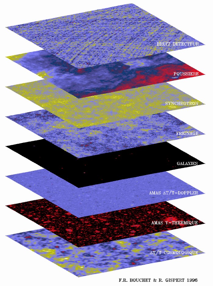
In Section 2.4.1, we saw how foreground emission from our own galaxy obscured the CMB at high and low frequencies. As the fluctuations in the CMB are at a level of less than 1 part in 10⁴, foreground emission is a much bigger problem when measuring the fluctuations in the CMB than when simply measuring the overall brightness to get the spectrum (Fig. 2.34).

Figure 2.34: The CMB fluctuations (bottom) have to be separated from many other components in the sky maps: from top to bottom: detector noise and artefacts, emission from dust, cosmic rays, and gas in our own galaxy, point-like emission from distant galaxies and quasars, the Sunyaev-Zeldovich distortion of the CMB spectrum by clusters of galaxies (here separated into `kinetic' and `thermal' components.

In practice, we need to operate in the `window' between about 2 cm and 1.5 mm, where CMB fluctuations are brighter than most of the foregrounds, as long as we observe regions well away from the Galactic plane. The exception is in the damping tail, where the weak CMB structure is confused by the random scattering of numerous faint point sources, mostly quasars at wavelengths down to around 2 mm, and probably distant galaxies at shorter wavelengths.

At these optimum wavelengths, absorption in the atmosphere is always a problem: observations at 1 cm and below can be made from high, dry sites such as Mt Teide on Tenerife, but at higher frequencies we must go above the atmosphere, either on a balloon or on a spacecraft.

Unfortunately, the predicted angular scale of the peaks, $\le$1^o or $\le$0.02 radians, is not ideal for making very precise measurements. Telescopes have angular resolution (in radians) of $\lambda$/D, where D is the size of the aperture. We therefore require apertures of a few hundred wavelengths to make the resolution smaller (but not too much) than the structure we are trying to observe. Contrast this with the aperture size for a typical microwave horn antenna: a few wavelengths, giving a resolution of $\sim$ 10^o, as for COBE. Horn antennas have reception patterns which can be very accurately calculated, and have extremely low receptivity to emission at large angles from the pointing direction. In contrast, to get an aperture 100 wavelengths across, a parabolic dish reflector is needed, i.e. a traditional radio telescope. Most existing radio telescopes are too big for the task: for 1 cm wavelength, we need a dish at most a few metres across. Furthermore, the reception pattern of a dish antenna is never as `clean' as a single horn: its sidelobes are larger, and also harder to calculate from first principles or to measure directly. As one tries to build up a map of the sky by scanning the antenna across the chosen region of interest, it is hard to be sure whether a small fluctuation in the output represents a fluctuation in brightness in the pointing direction, or a sidelobe passing over a bright object.

The observational situation improves for much smaller angular scales, of a few arcminutes (10^-3 radians) and below. On these scales, the classic technique is to connect separate dish antennas to form a aperture synthesis array, such as MERLIN or the Very Large Array (VLA). This technique again allows very good control of sidelobes.

As a result of these constraints, in the aftermath of the COBE discovery observers closed in on the acoustic peaks starting with observations on both small and large scales, where existing instruments could be pressed into service. Among the first results were measurements on arcminute scales with synthesis telescopes, of which the most sensitive was an epic 600-hr observation with the Ryle Telescope in Cambridge, setting an upper limit comparable with the level detected by COBE, but on scales more than two orders of magnitude smaller. The lack of detection was expected, as the fluctuations on these scales should be strongly suppressed by damping. On the large-scale side, the Jodrell-Cambridge-IAC collaboration on Tenerife built a 33-GHz interferometer. Like the previous beam-switch experiments (Section 2.5.1), this was a transit instrument and built up sensitivity for each declination strip by observing for several months. An interferometer works by multiplying the voltage signals from two horns looking in the same direction. The reception pattern on the sky is then a set of interference fringes: thus, if a bright point source transits through the beam, the output will be a series of positive and negative peaks. More to the point for us, an interferometer is a `ripple detector': a ripple on the sky aligned with the fringes will give a strong signal, while ripples with other wavelengths or orientations will cancel, as they are viewed simultaneously in the positive and negative fringes. This makes interferometers very convenient for measuring C_l: the fringe spacing $\theta$ = $\lambda$/D where D is the baseline, so an interferometer is sensitive to l $\approx$ 2$\pi$D/$\lambda$. A practical benefit is that emission on scales much bigger than $\theta$, such as from the atmosphere, is cancelled very precisely, so that interferometers are much less sensitive to weather than beam-switch experiments.

The sensitivity of an experiment to C_l as a function of l is known as the window function. An interferometer has a very narrow window function, but this was typical for the early experiments to measure CMB fluctuations; for instance switched beam experiments like Tenerife filter out structure on scales larger than the separation between the positive and negative beams on the sky, which is typically not much larger than the beams themselves. Therefore the overall C_l spectrum was slowly accumulated by combining the results of many experiments, Initially the 33-GHz interferometer was operated with a 15-cm baseline^2.10, giving it sensitivity to structure on scales of $\sim$ 2^o. Later the baseline was increased to 30 cm to optimise its sensitivity for the first acoustic peak.

What angular scale and multipole does a 30-cm baseline at $\lambda$1 cm measure?

Answer

The fringe spacing is

= /D = 1/30 = 0.03 rad = 1.9^o

This corresponds to

l = 2×30 = 188

close to the first acoustic peak.

If you are wondering why we are effectively using l 2/ here whereas we quoted l / before, remember that here is a wavelength, which corresponds to two 'bumps', one positive, one negative.

Many other instruments were designed or adjusted to home in on the acoustic peaks in the late 1990s, including instruments sited at the South Pole and balloon-borne experiments, which can get high into the stratosphere, greatly reducing problems with atmospheric emission, at the cost of observing time measured in hours rather than months. Balloon experiments allow the use of bolometers, sensitive detectors for far infrared emission, that are competitive with standard radio astronomy receivers for wavelengths shorter than a few millimetres.

By 1996 evidence was beginning to appear from all these experiments for excess fluctuations on scales of around a degree, but it was hard to be sure that this was not due to systematic errors, or to ordinary astronomical objects such as quasars or features in the Galactic foreground. What was needed was a detailed map, rather than one dimensional scans.

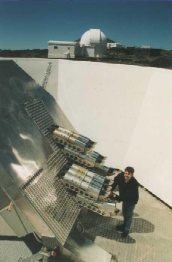
A classic way to make a radio map is via aperture synthesis, and several of the new instruments were miniature aperture synthesis arrays, starting with the Cosmic Anisotropy Telescope (CAT) at Cambridge. This was the first instrument to actually detect CMB fluctuations on scales smaller than the acoustic peaks, in 1996. The discovery map is shown on their web site. The CAT was the prototype for a more ambitious instrument called the Very Small Array (VSA), a joint Manchester/Cambridge/IAC project, sited on Tenerife (Fig. 2.35).

Figure 2.35: Left: The VSA under construction: 8 of the 14 microwave horns are laid out on a tip-table, which is housed in a large metal shield to keep thermal radiation from the ground from entering the horns. The peak of Mt. Teide is hidden behind the telescope dome in the background. Right: Close up of an `extended' configuration, with larger horns.

An aperture synthesis array like the VSA has a brightness temperature noise level of:

$$\Delta$$T = f

where T_sys is the system temperature, $\Delta$$\nu$ is the frequency bandwidth, i.e. the range of frequencies detected by the receiver, $\tau$ is the observing time, $\eta$ is a factor of around 2 quantifying various inefficiencies in the system, and f is the filling factor of the array, that is the fraction of the area of the array occupied by the antennas.^2.11 To maximise sensitivity (i.e. minimise $\Delta$T) we want to reduce the system temperature, which is related to the physical temperature of the receivers, maximise the bandwidth, and maximise the filling factor. As Fig. 2.35 shows, the VSA horns do indeed fill a larger fraction of the area they occupy. The VSA bandwidth is 1.5 GHz, large by previous standards (although its competitors use 10 GHz). Each horn has a compact cryostat to keep the receiver electronics at 15 K.

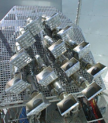
The optical design of the VSA is unique. The horns are each fronted by a 45^o mirror, making them resemble the original Bell labs horn. The array tracks the target patch of sky by tipping of the table on which the horns are mounted, and simultaneously rotating the horns about their long axis (Fig. 2.36). The horns can be reconfigured on the tip table: in the most compact configuration they are sensitive to multipoles between 200 and 900 (roughly the first three acoustic peaks), while spread out across the table they can reach l = 1800, allowing measurement of the damping tail.

Figure 2.36: Geometry of the VSA optics.

Like any synthesis array, the VSA is basically a collection of interferometers (we make one interferometer from each pair of horns). As the array tracks the target, the projected baselines seen by the target change; consequently the interference fringes produced by the target patch of sky steadily change their phase and rate. This is an important design feature, as the inevitable spurious signals in the system do not change in the same way, and so can be separated from the wanted sky signal. As well as the main array, the VSA system includes a system for measuring point source contamination in its target fields. This is a single-baseline interferometer using two large TV satellite dishes as antennas, separated by about 10 m. The long baseline and large collecting area make this much more sensitive to point sources, and much less sensitive to smooth fluctuations, than the main array. Once the point sources have been accurately measured, their effects can be subtracted from the data from the main array.

Two other CMB arrays have been built: DASI, at the South Pole, and the CBI, on the plain of Chajnantor, at altitude 16,400 ft in the Chilean Andes. Like the VSA they operate at $\lambda$1 cm. These two projects share a common design except that DASI has shorter baselines, designed for the first three acoustic peaks, while the CBI has longer baselines, designed to observe the damping tail. They are simpler than the VSA in that the individual horns do not track: they are mounted flat on a table which is pointed in the required direction. As a result they are less protected against spurious signals, which produce large fixed-pattern artefacts in their maps. These artefacts can be removed by the simple expedient of subtracting maps from different regions of the sky so that the constant instrumental effects cancel. You might think it a problem that at best they can return pictures of two sky patches superimposed (one in negative), but as the aim is only to measure the statistical properties, the only real disadvantage is a $\sqrt{2}$ reduction in signal to noise.

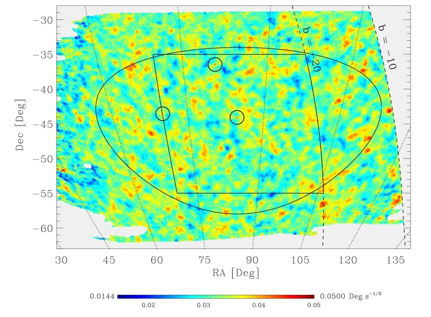
At the same time as these arrays were under construction, bolometer technology was improving rapidly, so that nowadays bolometers are the detectors of choice for wavelengths of 3 mm and shorter. In 1998 a balloon experiment called BOOMERanG was launched from McMurdo Sound in Antarctica. It carried a 1.3 metre off-axis telescope, with an array of 16 detectors horns at the prime focus, observing at five frequencies between 90 and 400 GHz (3 to 0.75 mm). The horns fed the photons to bolometers cooled to 0.3 K by a 60-litre tank of liquid helium. The theory was that the balloon would be caught up by winds high in the stratosphere which perpetually circle the pole, and make a circumnavigation of Antarctica, returning to the launch site after about 12 days. This was one in a long series of attempts to launch scientific balloons on long-duration flights from Antarctica, none of which had been entirely successful. But BOOMERanG did work. For more than 10 days the telescope collected high-quality data, eventually scanning a region about 30^o×50^o in size, roughly 3% of the sky. Eventually the experiment landed (intact) only 50 km from the launch site. The resulting map unequivocally showed the pattern of fluctuations in the CMB. For the first time, the clear dominance of a single scale size, the first acoustic peak, could be seen (Fig. 2.37).

Figure 2.37: The BOOMERanG map of the CMB sky. The three small circles surround three quasars detected faintly in the map; these three compact peaks show the resolution. Note that the characteristic size of the bumps is much larger. Outside the curved line (actually an ellipse, distorted by the map projection) the map is noisier because observed for a shorter time (left side) or contaminated by foreground emission from our Galaxy (right side; notice the excess of positive peaks). The lines marked b = - 10, b = - 20 (degrees) refer to Galactic latitude, i.e. distance from the Galactic plane.

The BOOMERanG results were announced in April 2000, at the same time as another balloon experiment called MAXIMA, which flew even more sensitive detectors but for a `normal' flight of about a day. The two sets of results agreed with each other, although the BOOMERanG results were more impressive from the longer flight time and the larger region of sky covered. By comparing the images at several frequencies, the BOOMERanG team could show that the fluctuations had a black-body spectrum, so that they belong to the CMB rather than to any Galactic foreground (although some Galactic contamination appears on the map, close to the Galactic plane). Great excitement was generated, not only by the clear discovery of the first peak, but by the apparent absence of the second. Theorists trying to fit the data found that this required a high baryon density, apparently contradicting the results from Big-Bang nucleosynthesis. However a year later the BOOMERanG team significantly revised their results, having spent the intervening time improving the calibration and data reduction. With this revision, a second peak was marginally detected, with about the amplitude originally expected. At the same meeting, the DASI team released their first results, which were in close agreement with the new BOOMERanG values.

The three CMB synthesis arrays were scooped by BOOMERanG for the first clear maps, but all have now announced their first results. Despite the very different observing techniques, and the large difference in observing frequency between the arrays and the balloon experiments, they all give consistent results for the statistical structure of the CMB (as yet, no two experiments have observed the same patch of sky, so only statistical properties can be compared). The joint results for the C_l spectrum are plotted in Fig. 2.38.

Figure 2.38: The observed angular power spectrum of the CMB from BOOMERanG, DASI, and the VSA, in May 2002. The smaller error bars on the BOOMERanG and DASI points show random errors; the larger ones show systematic errors which would lift or depress all points together. For the VSA such systematic errors are smaller than the random errors and included in the one error bar.

The combined results constrain the cosmological parameters in a way we could only dream about a few years ago:

Figure 2.39: The results of the Supernova and CMB cosmological tests are summarised. The solid and dashed contours show the region in the $\Omega_{m}^{}$, $\Omega_{\Lambda }^{}$ plane allowed by the two sets of supernova data. The blue diagonal region is the one allowed by BOOMERanG and MAXIMA data. The region allowed by both is cross-hatched. NB. the axes here are flipped compared to the ones in our Applet 1.12.

• The first acoustic peak is very well defined, peaking at l = 206±6, corresponding to a scale of about half a degree (the size of the Sun or Moon in the sky). This value is extremely sensitive to the curvature of the universe, and the result implies that space is almost exactly Euclidean (`flat'). The best-fit value for the overall density parameter is $\Omega_{0}^{}$ = 1.00±0.03.
• There is strong evidence for a dip followed by a second peak at l $\approx$ 550, and possibly a third at l $\sim$ 850. The height of these peaks relative to the first and each other strongly constrains the baryon density to $\Omega_{b}^{}$h² = 0.02±0.01, and weakly constrain the matter density to $\Omega_{m}^{}$ $\approx$ 0.34 (assuming a Hubble constant H₀ = 72±8 kms^-1Mpc^-1, taken from the Hubble Telescope results).
• The CBI results in particular support the idea of damping at higher l.
• Combined with the COBE data, the slope of the primordial power spectrum can be constrained: n = 0.91±0.1, to be compared with the scale-free prediction n = 1.

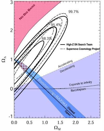Taken together with the evidence against a critical density in matter from studies of the large-scale structure (Section 1.4.3), the value $\Omega_{0}^{}$ $\approx$ 1 implies the presence of dark energy such as a cosmological constant or quintessence, quite independently of the direct evidence for an accelerating expansion from the supernova Hubble diagram (Section 1.4.5). These three lines of evidence together strongly point towards a `concordance model universe', Fig. 2.39, with

• $\Omega$ = 1
• $\Omega_{m}^{}$ $\approx$ 0.3
• $\Omega_{\Lambda }^{}$ $\approx$ 0.7
• $\Omega_{b}^{}$ $\approx$ 0.04
• H₀ $\approx$ 70 kms^-1Mpc^-1

2.6.4 Structure then and now

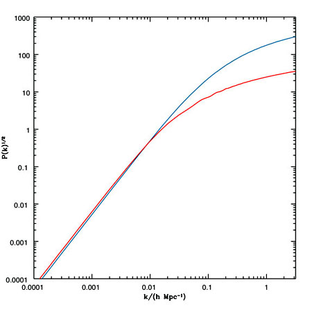
The density fluctuations in the early universe observed as structure in the CMB should have grown to produce the cosmic web of filaments and clusters of galaxies that we observe today via redshift surveys of galaxies. Obviously, the redshift surveys are showing us a different part of the cosmic web, in our cosmic neighbourhood as opposed to the edge of the observable Universe where we see the CMB fluctuations, so we can compare only the statistical properties of the structure, not individual features. But this is an important consistency check: although we are studying departures from pure homogeneity, we have every reason to expect that a statistical homogeneity remains; the probability of forming structures on a given scale, with a given amplitude, remains constant everywhere in the Universe.

These probabilities are encoded in the power spectrum of the large-scale structure (Section 2.6.1) and in the angular power spectrum (C_l spectrum) of the CMB (Section 2.6.2). The crucial point is that the fine-scale fluctuations we see in the CMB are on the same co-moving scales (20-200 Mpc) as the large-scale structure visible in the local universe. The CMB data give both the amplitude ( 2×10^-5 and the slope n $\approx$ 1.0 of the primordial power spectrum. We can `easily' evolve this forward in time to the present day on scales larger than 30 Mpc, where the fluctuations are still in the linear regime. With the help of large-scale computer simulations we can also estimate the effect of non-linear evolution on smaller scales. Fig. 2.40 show that the predicted power spectrum is in good agreement with the observed power spectrum derived from large galaxy surveys in the local universe: to within a factor of 2 on scales between 1 and 200 Mpc. It should be possible to make a much more precise test in a few years time, as the results from large galaxy surveys become available.

Figure 2.40: Power spectrum of the present-day matter fluctuations. Solid line: prediction from the best-fit model to the CMB fluctuations. Shaded area: uncertainty in the prediction. Points with error bars: observed power spectrum from the APM Galaxy Survey. NB. the different slope of this plot compared to Fig. 2.30 is due to a different way of defining the amplitude. Credit: John Peacock and the 2dFGRS team.

2.6.5 MAP and Planck: towards Precision Cosmology

The new frontier of CMB astronomy is to measure the C_l spectrum with much higher precision, and to detect polarization. This is not simply adding another decimal place:

• Most inflationary models predict that the primordial fluctuation spectrum is not precisely scale invariant. But different models predict different values for n (even the sign of the departure from n = 1 is up for grabs). Future experiments should be able to measure this deviation and so for the first time give evidence for or against specific physical models for inflation.
• Careful measurement of the damping tail will provide an independent cross-check on some of the cosmological parameters (e.g. the baryon density) derived already from the first few acoustic peaks.
• As we have seen, polarization provides a fundamental test of our theory of the CMB anisotropies, and also can measure any early re-ionization of the intergalactic medium, in which case we would be seeing the CMB through a later fog, and the cosmological parameters quoted above would have to be revised.

To make such precision measurements, we need to map not just a few percent of the sky, as done by BOOMERanG, DASI and the VSA, but all of it. The problem is that the CMB fluctuations are a random process. Cosmological models predict the width of the statistical distribution of fluctuation amplitudes, but any one fluctuation is a random sample from this distribution. The usual rule of statistics applies, that with N samples, you can measure the width of the distribution to a precision of 1/$\sqrt{N}$. So to get 1% precision, for instance, we would need 10,000 samples. In many situations we can get as many samples as we like, if we are patient enough, but with the CMB, each bump (or dip) on the sky corresponds to a `sample', which gives a fundamental limit to N. If we observe a small patch of sky, say the VSA field of view, with a diameter of about 4^o, then if we are interested in bumps on scales of 1^o, we have around 16 samples, giving at best 25% precision. If we analyse the same data for ripples on scales of 0.1^o we have effectively 1600 samples, giving 2.5% precision for small-scale ripples. Once the ripples are clearly detected, say with a signal-to-noise ratio of a few-to-one, there is no point in spending more time observing this region: although we could get improved measurements of the amplitude of each ripple, we will not learn any more about the underlying probability distribution.

Because the surface of last scattering has only a finite surface area, even a whole-sky view gives a finite precision. This limit is known as Cosmic Variance. We have been a bit vague about what we mean by a `ripple' up to now, but for an all-sky map it is easily specified: we are trying to determine the $\sqrt{C_l}$ values, which are the widths (standard deviations) of the probability distribution of the amplitudes of the (2l + 1) spherical harmonics corresponding to each multipole l. Therefore the best possible precision for each $\sqrt{C_l}$ is 1/$\sqrt{2l+1}$. For instance, COBE's low resolution allowed it to measure multipoles l < 20. Even though COBE's sensitivity was quite low by modern standards, its values for l < 10 are definitive because the errors are dominated by cosmic variance. Fortunately the acoustic peaks occur in the range 100 < l < 2000 (at higher l we lose the signal due to damping). For l = 2000, this gives a precision of 1/$\sqrt{4001}$ = 1.6%. This is good, but we can do better. As the angular power spectra in Fig. 2.32 shows, the C_l values are predicted to change smoothly with l, so we can safely average the C_l values at high l in groups of say $\Delta$l = 50; this will increase the precision by a factor of $\sqrt{50}$ = 7.

Having decided to map the whole sky, we run into a second problem: our own Galaxy. Up to now, experiments to measure the acoustic peaks have observed well away from the Galactic plane, thereby largely avoiding contamination by foreground emission. COBE dealt with this problem by analysing only the part of the sky more than 20^o from the plane, but this removes nearly half the sky. Furthermore, even a small amount of contamination, such as expected even far from the plane, would affect the more accurate experiments now planned This means we must make observations at a range of wavelengths, allowing us to separate the CMB and the various sources of foreground emission by using their different spectra, as discussed in Section 2.4.1.

Figure 2.41: The Planck Spacecraft

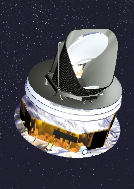
To get accurate maps of the whole sky, one has in practice to use a spacecraft, as was originally done by COBE. One such spacecraft, NASA's Microwave Anisotropy Probe (MAP) was launched in 2001 and is expected to announce results early in 2003. To find out more about MAP, see their excellent web site. A second mission is ESA's Planck spacecraft, due for launch in 2007.

Table 2.2 compares Planck and MAP. They share a number features. Rather than orbiting Earth, both will be positioned at the Second Lagrange point of the Earth-Sun system, known as L2. This is a point 1.5 million km away from Earth in the opposite direction to the Sun, where the gravitational fields of the Sun and Earth, and the centrifugal force, balance so that a spacecraft will orbit the Sun at the same rate as Earth.^2.12 The advantage of this position is that the Sun, Earth and Moon remain close together as seen from the spacecraft, so that it can always point its sensitive detectors away from all three simultaneously: they are all bright enough to affect the measurements even if only seen in the sidelobes. Both spacecraft will scan the sky by spinning, with their spin axis pointing towards the Sun, so that the detectors rapidly scan a circle on the sky. This circle gradually rotates as the spacecraft orbits the Sun, always keeping the sun behind it, so the whole sky is scanned each 6 months. Both spacecraft use small off-axis Gregorian telescopes to obtain the resolution needed to observe fine-scale structure in the CMB. The off-axis design means that the main mirror is not blocked by the secondary. Planck is shown in Fig. 2.41. Its focal plane is filled by two large arrays of detectors, the Low Frequency Instrument (LFI) consisting of radiometers (some under construction at Jodrell Bank) and the High Frequency Instrument which uses bolometers. MAP, like COBE, uses radiometers only: it is configured to measure the difference between two widely-separated positions in the sky, and so has two back-to-back telescopes. In contrast the Planck radiometers measure the difference between one sky position and an internal cold load. This is possible because unlike MAP, the Planck instruments are actively refrigerated, giving it the lowest operating temperature of any space mission to date.

Table 2.2: A comparison of the MAP and Planck Missions

Instrument	MAP	Planck
Launch	July 2001	February 2007
Mission lifetime	2 years	14 months
Orbit	L2	L2
Spin Period	2.2 minutes	1 minute
Telescope Diameter	1.4 m	1.5 m
Cooling	Passive	Active
Instrument		LFI	HFI
Wavelength range	13-3.3 mm	10-4.3 mm	3-0.35 mm
Number of bands	5	3	6
Detector type	Radiometers	Radiometers	Bolometers
Number of detectors	10	5	36
Operating Temp.	95 K	18 K	0.1 K
Best resolution	13 arcmin	14 arcmin	5 arcmin
Sensitivity /pixel	31 $\mu$K	12 $\mu$K	5 $\mu$K
Multipoles	1$\le$l$\le$1000	1$\le$l$\le$1000	1$\le$l$\le$3000

As the table shows, Planck will be a substantial improvement on MAP. It should be able to map the CMB fluctuations over nearly all the sky to an accuracy set by small-scale irregularities in the spectra of the foreground components, which will prevent us from separating them from the CMB with perfect accuracy. This should be the last word in measuring the CMB, except for polarization.

Although both MAP and Planck should be able to make a statistical detection of CMB polarization, neither will give us accurate maps (rather like the situation with COBE for temperature fluctuations). Polarization is certainly the new frontier of CMB science. Several ground-based and balloon experiments are racing MAP for the first detection, and concepts for a next-generation space mission to measure polarization are beginning to circulate. Watch this space!