2.4 The CMB and the history of the Universe

2.4.1 The spectrum of the CMB

Since its discovery, the spectrum of the CMB has been measured at a wide range of wavelengths. The best present-day data comes from three sources

• Ground-based measurements with radiometers operating at a single wavelength.
• Observations of interstellar CN, in the tradition of McKellar.
• at $\lambda$ < 3 mm, direct measurements have to be made from space. Because of the large cost of space experiments, they tend to measure a broad spectrum rather than just a single wavelength.

We will look at each of these in turn.

2.4.1.1 Ground-based Measurements

Ground-based measurements of the CMB spectrum still follow the basic technique used by Penzias & Wilson in 1965. The central tool is a radiometer, that is, a radio receiver designed to make accurate measurements of the input power level. Radiometers must view the sky through some sort of antenna, which has the job of selecting radiation from a small region of interest and rejecting it from the rest of the sky. This is described in terms of the beam pattern which is simply a map of the attenuation suffered by emission coming from each direction; in the centre (the pointing direction) we set the beam amplitude to unity, and it falls to a small fraction at angles more than the beamwidth away from this. The beamwidth is set by diffraction at the antenna aperture, $\theta$ $\sim$ $\lambda$/D radians.

The Bell Labs horn had an aperture D of 20 feet, giving a beamwidth at 7 cm of around 0.01 rad or 0.8^o. It might be thought that the large aperture helped collect a lot of radiation to give a strong CMB signal, but the small beam meant that it only collected emission from a small patch of sky. For an extended source of emission like the CMB, the power received is proportional to the telescope collecting area times the angular area (solid angle) of sky to which the antenna responds, i.e. D²×($\lambda$/D)². In words, the size of the antenna is irrelevant when observing the CMB, except for a few practical considerations. A 20 foot antenna is not a very practical device to move around, and all subsequent experiments have used much smaller ones. Typically, the beam size is set at around 10^o, which is small enough that when you point away from the Galactic plane and from the ground, radio emission from these sources is strongly rejected. This is particularly important for the ground, because, in the radio, it is a good black body at about 300 K; a small fraction of this would be a serious contaminant to the 3 K CMB signal.

Antenna beams never fall exactly to zero; there are always secondary peaks at large angles called sidelobes (these are the equivalents of diffraction rings in optical telescopes). For precision experiments these must be as small as possible to avoid contaminating signals from the telescope structure, ground, and Galaxy, and for this the best plan is to use a very simple design, usually a simple corrugated horn at the end of a waveguide. The corrugations are a set of $\lambda$/4 grooves cut on the inside of the horn which help suppress the sidelobes. Antennas are often further protected by surrounding them with a reflecting ground screen so that the sidelobes view (in reflection) the cool sky rather than the warm ground.

Another major problem is emission from the atmosphere. Although the optical depth $\tau$ of the atmosphere is rather low at frequencies up to about 140 GHz ($\lambda$2 mm), the temperature, T $\approx$ 300 K, is a hundred times higher than that of the CMB. Recalling from Section 2.1.1 that the intensity of a partially transparent screen is $\tau$B($\nu$, T), so the brightness temperature is just T_B = $\tau$T, we can see that even a modest optical depth is a problem. Atmospheric mm-wave emission is dominated by oxygen (large amplitude but stable) and water vapour (smaller but highly variable). The water vapour is the main problem as its emission is too unpredictable to easily subtract out. To avoid it, modern ground-based CMB experiments are made at high, cold sites, where the atmospheric water is frozen (ice crystals, as in cirrus clouds, are much less of a problem than vapour).

Finally, we have to deal with radio emission from our Galaxy, which is present all across the sky, although concentrated near the Galactic plane. Several different components of the interstellar material contribute:

• Very rare, but very energetic, electrons with v $\approx$ c, one component of the cosmic rays, emit synchrotron radiation due to their spiralling motion in the interstellar magnetic field. This has a roughly power-law spectrum with T_B $\propto$ $\nu^{-2.8}_{}$.
• A substantial fraction of interstellar space is filled with ionized gas at temperatures of around 8000 K. Electron-proton collisions here emit so-called free-free radiation, also known as bremsstrahlung. This is a form of thermal radiation. At radio frequencies $\tau$($\nu$) $\propto$ $\nu^{-2.1}_{}$. Combined with the low-frequency limit of the black body spectrum B_RJ($\nu$, T) $\propto$ $\nu^{2}_{}$, this gives a brightness temperature T_B $\propto$ $\tau$B $\propto$ $\nu^{-0.1}_{}$.
• Another large fraction of space is full of neutral gas with temperature < 100 K. In these cold regions heavier elements like carbon, nitrogen, oxygen, and iron condense to form sub-micron sized grains, the interstellar dust. This dust has a negligible optical depth to radio and microwaves, but at millimetre and sub-mm wavelengths around the CMB peak, $\tau$ rises rapidly with frequency, giving roughly T_B $\propto$ $\nu^{4}_{}$.

Rising synchrotron emission towards low frequencies, and dust towards high frequencies, make the CMB spectrum difficult to measure far away from its peak; in practice it has not been detected at wavelengths longer than 50 cm or shorter than 0.4 mm. But we should count ourselves fortunate that the CMB peaks at frequencies where the Galaxy's spectrum is close to a minimum, so here at least we have a clear view. Galactic emission is dealt with by the simple but tedious expedient of making measurements at a series of low and/or high frequencies, where it is the main component, and extrapolating to find the necessary small correction at the frequency where we are trying to measure the CMB.

Ground-based measurements are important in the microwave band, where the atmosphere is still highly transparent and the CMB is not yet swamped by Galactic synchrotron emission.

2.4.1.2 Observations of Cyanogen

As we saw in Section 2.2.1, the cyanogen (CN) molecule functions as a detector at $\lambda$2.64 mm, because photons with this wavelength provide the energy to give the molecule one unit of rotation. In addition, a second unit can be added by photons with $\lambda$1.32 mm. The rotational state of the molecule can be deduced from absorption lines in the optical spectra of nearby stars. Modern CCD detectors giving accurate, linear, measurements of the light levels, now easily detecting the very faint lines from the second rotational state. To get a really accurate measurement of the radiation field at these wavelengths, it is no longer enough to pretend that the molecules are sitting isolated in space. Although the density is very low, from time to time they collide with other electrons or atoms, and these collisions can also set them spinning. This effect contributes an effective `local' temperature T_loc. Fortunately, the molecules also emit $\lambda$2.64 mm photons as they revert to their non-rotating state, and this emission depends only on T_loc. Observations of the millimetre emission line allow this to be calculated for each line of sight. The best data is still from the original star zeta Ophiuchi, and the latest measurements for this and other stars give T_loc typically a few tens of mK or less.

With these corrections made, the latest results from CN are remarkably accurate:

T_CMB = 2.729±0.03 K      ($$\lambda$$2.64 mm)

T_CMB = 2.656±0.06 K      ($$\lambda$$1.32 mm)

A skeptic might note that these results were published just after the direct measurement by FIRAS on board COBE; somehow accurate results are easier to get when you already know the answer!

2.4.1.3 Observations from space: FIRAS

Although there have been a number of space experiments to measure the CMB spectrum, the Far Infrared Absolute Spectrometer (FIRAS) on the Cosmic Background Explorer (COBE) produced by far the best data, and we will look at this instrument in detail.

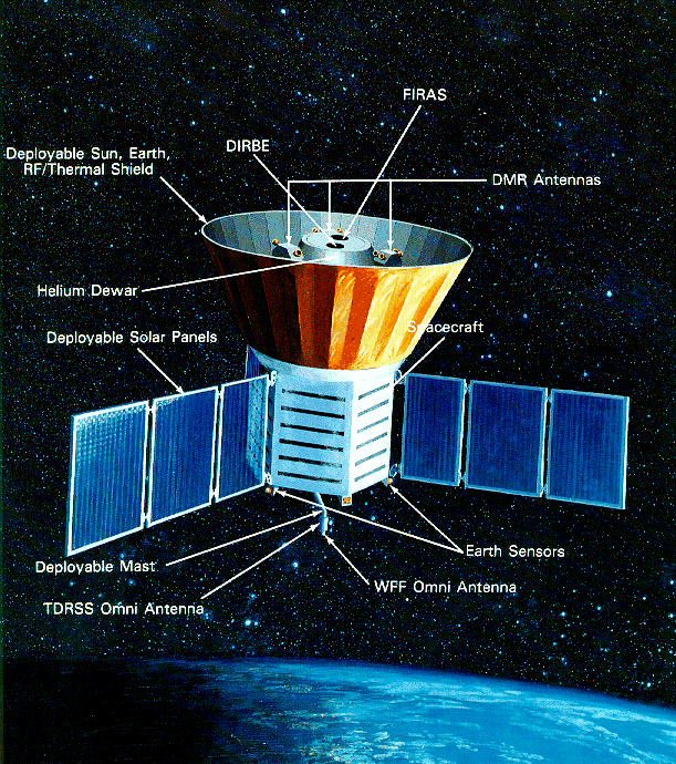
The COBE satellite is shown in Fig. 2.9. It carried three scientific experiments: FIRAS, DIRBE (an infra-red experiment), and the DMR (discussed in Section 2.5.1). FIRAS and DIRBE were installed in a dewar (sophisticated thermos flask) of liquid helium. Gradual evaporation of the helium limited the lifetime of these instruments to ten months in 1989-90. The data collected in this period is still definitive.

Figure 2.9: The Cosmic Background Explorer (COBE) Satellite.

COBE had a nearly polar orbit, designed to slowly precess so that it stays approximately perpendicular to the direction to the Sun; in other words, the orbital plane was Earth's day/night terminator. The satellite spun at just over once a minute around its symmetry axis, which is also the direction that FIRAS points. This axis was kept pointed roughly away from Earth and at right angles to the Sun, so that the observing direction tracing out a great circle on the sky. As the Earth travels along its orbit, the direction to the Sun, and hence the scanned circle, slowly rotates, so that after six months the whole sky was covered.

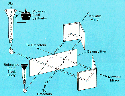
FIRAS observed the sky through a trumpet-shaped horn which gave a beamwidth of about 7^o, across a wide range of frequency. The spectrum was measured in an apparently roundabout manner: the CMB radiation was split two ways and then recombined to give an interference pattern (Fig. 2.10). The total intensity was measured by broad-band detectors (bolometers) while the mirrors in the interferometer were moved backwards and forwards, changing the length of the radiation paths. Once we known the intensity for each value of the length difference between the two paths, the spectrum (i.e. intensity as a function of frequency) can be calculated: the interference pattern is the Fourier Transform of the spectrum. There are several advantages to this method. First, Fourier transforms are related to holograms: each data point on the interference pattern encodes information from the whole spectrum, and vice versa. The effect of this is that an error or dropout in the raw data will not affect a single frequency in the spectrum, but will change the overall amplitude, largely preserving the spectral shape, which is of more interest than the amplitude, as we will see.

Figure 2.10: Block diagram of the Far Infrared Absolute Spectrometer (FIRAS) on board COBE.

FIRAS also included a double system of calibration. As well as the sky horn, radiation from an internal calibration source was passed through the interferometer, and the output of FIRAS was the difference between the sky and internal signals: the temperature of the internal calibrator was adjusted to make this nearly zero. This has the same effect as switching against a cold load in a standard radio receiver: many systematic errors are automatically cancelled out. But because the light path from the internal calibrator was not exactly the same as that from the sky, and the calibrator itself was not a perfect black body, some systematic errors remained. The definitive calibration was done using a cold plug, much like a trumpet mute, that could be swung in to the end of the sky horn. The plug was an almost perfect black body (absorbing 99.95% of the radiation that fell on it at FIRAS' operating frequencies). The temperature of this calibrator was monitored very carefully, and so the output of FIRAS with the calibrator in place was known to correspond to black-body radiation with a known temperature. The calibrator was inserted many times during the mission, allowing small changes in the instrumental response to be measured. The result was the most precise measurement of the CMB temperature to date, with a very conservative error of 2 mK. Even so, the relative brightness at different wavelengths and in different directions on the sky is known far more accurately than this; the absolute scale is limited by uncertainty in the precise temperature of the calibrator.

2.4.1.4 Experimental results

Fig. 2.11 shows the best experimental data on the CMB spectrum. All the data is fitted to within the errors by a black body spectrum with

T_CMB = 2.725±0.002 K

Compare this with the other astronomical spectra in Fig. 2.2. Although I chose objects with relatively smooth spectra, the CMB spectrum is by far the smoothest. Not only that, but it is fitted to within the very small experimental errors by a perfect Black Body spectrum.

Figure 2.11: Left: measurements of the spectrum of the CMB. The dashed curve is a theoretical Black Body with T = 2.7253 K. Right: Brightness temperature as a function of frequency, to show the residuals. Colour coding is the same as the first plot.

2.4.2 How far away is the CMB?

In Section 2.3 we saw how the CMB was produced according to the standard Big Bang theory. In this section we will ask what we can deduce directly about the distance to the CMB "emission" surface, and hence about the time it was produced.

The black-body spectrum of the CMB tells us we are completely surrounded by material with a very high optical depth; as we have seen (Section 2.1.1), this requires a lot of stuff. The form of the spectrum appears to tell us that the emitter was at a temperature of 2.725 K, but there is a catch. If the emitter is at a large distance, the light will be redshifted.

Because of the unknown redshift, we can't directly tell the temperature or the distance of the "wall" that surrounds us. From the isotropy of the CMB, to be discussed in Section 2.5.1, we can tell that at any given redshift back to the emitting wall, the temperature was the same in all directions. Furthermore, if the `wall' is fuzzy, so that the photons are emitted over a range of redshifts, the temperature during that period must track the cosmological expansion T $\propto$ (1 + z), or we would see a range of temperatures superimposed, not a pure black body. This isotropy makes it most likely that the wall must be at the same redshift, hence the same distance, in all directions.

At first sight this puts us in the centre of an isotropic but very inhomogeneous universe. But there is a more palatable alternative: we know that the universe changes with time, and as we look out to higher redshifts we are looking back in time. The distance to the CMB wall may actually be the distance a photon can travel since a time when the universe was opaque everywhere; more precisely, the time when the universe changed from being opaque to transparent, so that ever since the photons have travelled freely. For this reason the wall of the CMB is known as the surface of last scattering. Of course this name assumes, following the standard theory, that there was a long period of scattering after the actual production of the photons.

2.4.2.1 Holes in the microwave background

There is one rock-solid constraint on the distance to any object: it must be beyond anything which can be seen to get between the object and us. The CMB comes from every direction, so you might think it would be easy to find something in front of it, but there is a problem. To be sure the obstacle is in front, it has to block the CMB photons, (at least a fraction of them), so we are looking for a "hole" in the CMB. But if the object itself radiates, its own emission will fill in the hole. We have seen that good absorbers, objects with a high optical depth, are also good emitters and will radiate with their own temperature. As far as we know, nothing in the Universe is significantly cooler than the CMB, so apparently we will always see a brightening, not a dimming. And skeptics will claim that in fact the bright object is seen behind the CMB "wall", arguing that the wall is partially transparent.

But there is an escape clause, noticed by Russian astrophysicists Rashid Sunyaev and Boris Zel'dovich. We can look for cases where the obstacle does not absorb the CMB photons, but simply scatters them. This is what happens when CMB photons pass through the low density ionized gas that fills intergalactic space. Occasionally, a photon will collide with an electron. In the collision, the total momentum and energy of the particles is conserved, but their directions are changed and typically some energy is transferred from the higher-energy particle to the lower-energy one; that is, from the hotter to the cooler. Since the CMB photons are cooler than practically everything else, they generally gain energy in collisions. This process is called inverse-Compton scattering.^2.5If enough photons are involved in collisions, the overall spectrum of the CMB will be measurably distorted.

The ideal place to look for this Sunyaev-Zel'dovich (or SZ) effect would be somewhere where there is a lot of ionized gas, and where the gas was very hot, to maximize energy transfer so that the distortion of the CMB spectrum is easy to see. To avoid masking the effect on the CMB spectrum, the gas must produce essentially no radiation of its own at microwave frequencies, and that requires very low densities.

Clusters of galaxies fit the bill. The gas between the galaxies is the hottest of all intergalactic gas, with temperatures up to 10⁸ K. There is a huge quantity of it: as we saw in Section 1.4.3, typically ten times as much as all the stars in the galaxies of the cluster. The gas shines brightly in X-rays, but its density is low enough that there is no detectable emission in microwaves. Despite the large mass of gas, the chance of collision for any given photon is less that 1% for even the biggest clusters. Photons enter the cluster from all directions, so although some photons are scattered out of our line of sight, others are scattered towards us; the total number travelling in each direction is unchanged. Only, a small fraction of them have gained energy in collisions with cluster electrons. The effect on the spectrum is shown in Fig. 2.12. Essentially, the whole spectrum is shifted slightly to higher energy.

Figure 2.12: The Sunyaev-Zel'dovich (SZ) effect. Left: CMB photons enter the cluster from all directions; the small fraction scattered to higher energy (symbolized by blue photon symbols) leave the cluster in all directions. Right: the Black Body spectrum on entry (red solid line) is slightly shifted to higher frequency $\nu$ on exit (blue dashed line).

If the excess above the peak of the spectrum were all that was detected, it might be attributed to some unknown emission process in the cluster. But below the peak we see a decrement, the "hole" in the CMB that we have been looking for. This can only happen when the cluster is in front of the CMB emission zone. The decrement is small: the largest values are a few millikelvin (mK) or around 0.1% of the CMB temperature, as you might expect from the fraction of photons scattered.

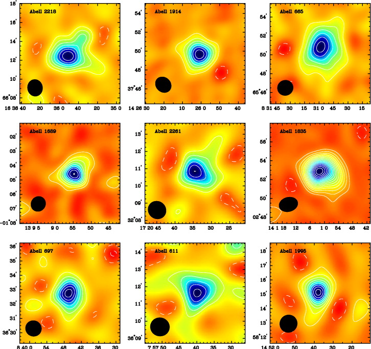
The prediction of this effect by Sunyaev and Zel'dovich (1970) prompted a long series of attempts to detect the decrement, which stretched radio telescopes to their limits. Early results were controversial and mainly turned up systematic errors in the measurements. Moreover, although the cluster gas does not itself emit microwaves, many clusters turned out to contain microwave-emitting radio galaxies and the still-mysterious radio haloes, which masked the decrements. But by the mid-1980s the effect had been detected in three clusters by several independent groups, typically with hundreds of hours of observations on each cluster. Nowadays it can be detected in an afternoon by telescopes designed to search for the intrinsic fluctuations in the CMB, which are much fainter than the SZ decrements. Some recent results are shown in Fig. 2.13. The highest-redshift cluster with a secure SZ decrement is at z = 0.83; this confirms that the CMB is a genuinely cosmological signal and not, as some doubters once suggested, a local "fog" produced near or even in our own Galaxy.

Figure 2.13: Observations of the Sunyaev-Zel'dovich (SZ) effect. The black ellipses show the instrumental resolution. From Grego et al. (2001).

2.4.2.2 Quasars and the CMB

The object with the highest reliably-known redshift is a galaxy at z = 6.56. If the CMB "wall" was truly optically thick, it would have to be at a higher redshift than this. But the known objects at the very highest redshifts have not been detected at wavelengths near the peak of the CMB, so it can (and has) been argued that the CMB only has a high optical depth in this band. In particular, Fred Hoyle and a few others have recently developed a `Quasi-Steady State Cosmology' in which, as in Dicke's early 1960's model, the Universe oscillates in size. In the QSSC the collapse never reaches early-universe densities, and so it is proposed that the CMB consists of starlight, mostly from the previous cycle, which has been absorbed by interstellar grains and re-radiated as a black-body at z $\approx$ 5. The 'grains' needed to do this are essentially small radio aerials: mm-long fibres of iron and other metallic elements. These are designed by Hoyle et al. to have a high optical depth near the CMB peak, but should become transparent at wavelengths of around 20 cm (where, in fact, we can no longer accurately measure the CMB spectrum).

Let's quantify this. The brightness of a source with physical temperature T_ph and optical depth $\tau$($\nu$) is

I($$\nu$$) = (1 - e^{- $\tau$}) B($$\nu$$, T_ph).

An object behind the emission layer would have its brightness reduced by a factor e^(-$\tau$). Show that in the Rayleigh-Jeans regime, i.e. when h$\nu$ $\ll$ k_BT, this is equal to $\Delta$T/T_ph, where $\Delta$T is the difference between the physical temperature and the observed brightness temperature.

Answer

In the Rayleigh-Jeans regime, intensity I T_B. By definition the brightness temperature of a black body at temperature T is T_B = T, so our formula can be written

T_B = (1 - e^- )T_ph = T_ph - e^- T_ph

Re-arranging:

e^- T_ph = T_ph - T_B = T

i.e.

e^- = T/T.

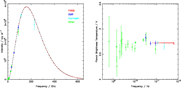
The CMB has the best black-body spectrum found in nature; I($\nu$) = B($\nu$, T_CMB) to within 0.03% from 60 to 600 GHz. The natural explanation is that T_ph = T_CMB (allowing for redshift as previously discussed), and $\tau$($\nu$) > 8 ($\tau$ > 10 around the peak at 200 GHz). Otherwise, to simulate a black body spectrum, we would need T_ph > T_CMB and $\tau$($\nu$) varying in exactly the way needed to compensate for the different shape of B($\nu$, T_ph) and the observed spectrum B($\nu$, T_CMB). It is very unlikely that any substance would have such a contrived variation of optical depth.

Figure 2.14: Radio spectra of the quasars PKS 2000-330 at z = 3.773 (black squares) and B31428+422 at z = 4.715 (open circles). This sort of "flat" spectrum is typical for radio-bright quasars. The discrepant points in these spectra are almost certainly due to variability of the quasars, as the data was taken over a number of years. Data from the NASA Extragalactic Database (NED).

Let's take it that $\tau$ is high around the peak of the CMB spectrum. Any object behind the wall would vanish when observed at frequencies around the CMB peak, or at least dim by a very large factor. In fact, a number of quasars with redshifts up to z $\approx$ 5 have been observed between 1 and 10 GHz (e.g. Fig. 2.14). In this band, the limits on $\tau$ are less good: a number of measurements in Fig. 2.11 between 3 and 10 GHz are below the FIRAS temperature by around 0.08 K. Although this discrepancy is not formally significant, it is consistent with a finite optical depth of $\tau$ $\approx$ 3.5.^2.6 If our high-redshift quasars were behind the CMB emission region, we would expect an attenuation by a factor of 0.08/2.7 = 0.03. In the QSSC cosmology, the CMB should get more transparent at lower frequencies, so we would expect a rather dramatic decline in brightness with frequency in Fig. 2.14, whereas the observations show a change of less than a factor of 2, which could easily be the true shape of the spectra. This is strong evidence that the CMB emission zone is more distant than z = 4.7.

In the last few years it has become possible to detect luminous quasars and star-forming galaxies at z > 4 at sub-mm wavelengths, close to the peak of the CMB. The emission is believed to be due to dust at temperatures of a few ×10 K, and the spectra are typically steeply rising to shorter wavelengths. These objects show a minimum in their spectrum near the observed CMB peak, conventionally interpreted as a valley between dust emission at $\lambda$ < 1 mm and emission from ionized gas which dominates at longer wavelengths. This minimum looks vaguely like the absorption notch expected from a foreground "CMB layer"; but if we correct the spectrum on the assumption that such a layer has a minimal optical depth of $\tau$ = 10 near the peak, the luminosities required are phenomenal... No objects this bright are known at lower redshifts.

How much would we have to increase the observed brightness by to allow for an optical depth of 10?

Answer

For = 10, we have attenuation by a factor of e^-10 = 4.5×10^-5. To find the true brightness we would have to divide out this attenuation factor, i.e. multiply by e = 22, 000.

In short, with very simple arguments we can push the CMB back to redshifts nearly as high as the most distant known object. To go much further than this we have to assume the Big Bang cosmology, and rely on the self-consistency of all its implications to re-assure us that our assumptions were correct.

2.4.2.3 Ancient thermometers

The prediction that the CMB temperature increases with redshift in proportion to (1 + z) can be directly tested by using the same sort of absorption-line analysis as was done by McKellar in 1941 (Section 2.2.1). Distant quasars are used as the background light source instead of the nearby star used by McKellar. Gas clouds in front of the quasar cause absorption lines in the observed spectrum, and analysis shows the temperature of the gas. These measurements are difficult and mostly yield only upper limits to the CMB temperature (all greater than (1 + z)T_CMB!), but in two cases actual temperature measurements are possible. In the first, at z = 1.776, there are two clouds with slightly different velocities, and excitation temperatures of 10.4 K and 7.4±0.4 K (Songaila et al. 1994). Obviously, the gas in the first cloud has an additional heat source. In principle there could also be another heat source for the second cloud, so the observation of a higher CMB temperature is not absolutely water-tight in this case. In the second case, at z = 2.338, absorption lines are seen from neutral carbon, singly-ionized carbon, and the hydrogen molecule. Together, these rule out alternative heat sources and give a CMB temperature 6 < T < 14 K (Srianand et al. 2000).

What are the predicted CMB temperatures in these two systems?

Answer

At z = 1.776, T = (1 + z)T₀ = 2.776×2.725 = 7.565 K in very good agreement with the measured temperature of the second cloud. At z = 2.338 we should have T = 9.096 K, in the middle of the range of temperatures allowed by the observation.

2.4.3 What can we learn from the CMB spectrum?

2.4.3.1 Early energy release

As we learnt from the confusion caused by Fabry's temperature of space (Section 2.1.4), the CMB contains a rather similar energy density to that of starlight in the Milky Way. But if we subtract out this local emission and consider a random point in the universe, typically deep in intergalactic space, the CMB turns out to carry around 90% of the energy density of all photons (Fig. 2.15).

Figure 2.15: Intensity of extragalactic light between radio and ultraviolet wavelengths. The grey peak is the CMB, while the blue and red data points and the purple upper limits are measurements of the far-infrared and optical background light. There is some disagreement between the data points due to different estimates of the Galactic emission which has to be subtracted to reveal the remaining extragalactic light. The green curve is a model for these backgrounds: the peak near 1 micron is the accumulated starlight that escapes from galaxies over the history of the Universe. About a third of the starlight is absorbed by dust and re-radiated in the far infrared, giving the middle peak. The numbers give the intensity of each component. Credit: Ned Wright. See his Cosmic InfraRed Background Page for full details.

Furthermore, the remaining 10% of the photons are mostly produced by stars over the history of the Universe,

This simple observation rules out many cosmological possibilities, in which large amounts of energy were released at early times. For instance, if one of the components of the dark matter was made of an unstable particle with a life short compared to the age of the universe, a large amount of energy would be released in the form of photons with a very non-thermal spectrum. No such energy release could have happened since the CMB spectrum was frozen about 40 years after the Big Bang. (Recall that at this time electron energies become so low Compton scattering ceased). Nor could a large amount of energy have been dumped directly into the baryonic matter that was scattering the CMB photons: this would have energised the electrons enough so that Compton scattering started again and some of this energy would then be transferred to the CMB, giving a characteristic Comptonised spectrum, just as in the SZ effect. The lack of this type of distortion on most lines of sight limits any such energy release before last scattering to < 5×10^-5 of the energy in the CMB.

But there is more. Suppose some large amount of energy was released earlier than t =40 yrs. Compton scattering would have blurred out the spectrum of the newly-generated photons, sharing their energy with the ones already in the CMB, and so producing something roughly like a black body spectrum, but not exactly the same. In a true black body both the energy density and the photon number density are fixed by the temperature. Non-thermal energy release would not respect this relation, and scattering preserves both energy and number density (or rather, it does not affect the way these change with redshift). The net effect of Compton scattering is to produced what is called a Bose-Einstein spectrum. The CMB data has been fitted to the Bose-Einstein formula, and we find that < 6×10^-5 of the CMB energy could have been added since thermal decoupling, just 5 days after the Big Bang.

Before this time, energy exchange between photons and particles was efficient enough that any energy release would just have raised the overall temperature, with the spectrum in a pure black body form. But there is still an important check: the calculation of Big Bang Nucleosynthesis is made assuming that the temperature a few minutes after the Big Bang is simply the redshifted version of the CMB we see. A large enough energy release after nucleosynthesis would spoil the rough (factor of 2) agreement between the baryon density derived from nucleosynthesis and the baryon density we observe today. Partridge (1995) estimates that at most the temperature could have been raised by a factor of 2.5 in this period.

2.4.3.2 Spectral lines in the CMB

During re-combination we have seen that electrons combined en masse with atomic nuclei. In this process, spectral lines are emitted, i.e. photons at the particular energies corresponding to the quantum jumps between energy levels in the new atoms, as the electrons drop down to the lowest energy level in each atom. Most of these atoms are hydrogen, and the normal way for an electron to reach the ground state is to emit a Lyman-series photon, most commonly Lyman-$\alpha$ which is emitted when the electron jumps from the second-lowest to the lowest state. The emitted wavelength of Lyman-$\alpha$ is 121.6 nm, so after being redshifted by a factor of 1100 to 1600, it should appear at 130-200 $\mu$m, in the far infra-red. In fact no such line has been detected and it is reasonable to ask why not.

On closer investigation, the failure to detect spectral lines from recombination is not surprising. First, there is only one atom per 10⁹ CMB photons, so the emission of a few photons per atom would not add very much (even though the typical energies are several times higher than those of CMB photons). Second, recombination took place over a fairly broad range of redshift, which will turn the spectral line into a broad hump, hard to distinguish from the general infra-red background, which comes from numerous faint galaxies at redshifts of a few. Finally Lyman photons have a special problem: unlike generic CMB photons, they have just the right energy to be absorbed by hydrogen atoms, and so, once recombination has begun and there are many hydrogen atoms around, a Lyman photon will almost instantly be re-absorbed. This promotes the electron in the absorbing atom back to the energy level at which emitting atom started, giving no net change. So in the conditions of the recombination era, for an electron to reach the ground state and not knock another electron back up, it has to arrive by an unusual route, for instance two-photon emission; in that case each photon has about half the energy of Lyman-$\alpha$ which is not enough to be absorbed by another atom.

As a result of all this the best chance for detecting spectral lines from recombination turn out to be the lines from trace elements such as lithium. Unfortunately even for these the predicted line strengths is well below what could feasibly be detected at present.