
T7 - Self-calibration of 3C277.1
This tutorial is designed to take you through the process of self-calibration of a 3C277.1 data set. By this point, you should have learnt about phase-referencing and imaging. This final step will teach you about removing the remaining antenna-based calibration errors that are typically induced by the differing atmospheric paths between your target and phase calibrator. To do this we need to use self-calibration. This is similar to standard calibration except that we do not assume that our calibrator is a point source (1 in amp-uv and 0 in phase-uv space).
Data download and accompanying presentation
To download the data required for this tutorial and the accompanying presentation, please use the following download links:
Move this dataset (tar -xvf 3c277_workshop_pt2_only_ERIS2019.tar.gz) into a suitable folder e.g. T7_self_calibration and untar the bundle using tar -xvf 3c277_workshop_pt2_only_ERIS2019.tar.gz. You should have the following files in your current directory before you start:
3C277.1_imaging_outline_E19.py- calibration script equivalent of the guide3C277.1_imaging_all_E19.py.tar- compressed script in case you get stuck1252+5634_E19.ms- partially calibrated measurement set1252+5634_1.clean.image- image of target with only phase referencing calibration appliedtarget.p1- initial pre-processing round of phase-only self-calibration applied to the datatarget.p1_L.png- plot of initial phase calibrator solutions (L correlation)target.p1_R.png- plot of initial phase calibrator solutions (R correlation)
Table of Contents
- Generate model for self-calibration (step 1)
- Inspect model (step 2)
- Inspect to choose interval for second phase self-calibration (step 3)
- Phase-self-calibrate again (step 4)
- Apply the solutions and re-image (step 5)
- Choose solution interval for amplitude self-calibration (step 6)
- Amplitude self-cal (step 7)
- Apply amplitude and phase solutions and image again (step 8)
- Reweigh the data according to sensitivity (step 9)
- Final image & multi-scale clean (step 10)
- Summary and conclusions
The task names are given below. You need to fill in one or more parameters and values where you see ***. Use the help in CASA, e.g. for tclean.
taskhelp                        # list all tasks
inp(tclean)                     # possible inputs to task
help(tclean)                    # help for task
help(par.cell)                  # help for a particular input (only for some parameters)
What has been done to this data
Due to time constraints in this tutorial, the data set you have received has has a lot of pre-processing applied. The following has been conducted:
- Firstly, all of the phase-referencing calibration that you have done in the previous tutorials has been applied to the target field (1252+5634)
- The parallel hand polarisations with the phase referencing corrections applied have been split into a new measurement set and extra averaging has been applied (8s, 64 channels per spw). This is so that the steps in this workshop can proceed quickly. In the imaging tutorial you should have made the first phase-referenced calibrated image of the target. You can inspect this for this tutorial by opening the
1252+5634_1.clean.imagein the CASA viewer. - An initial round of phase-only self-calibration has been conducted (using a solution interval of 180s) has been applied as described in the accompanying presentation. You can inspect the solutions applied by looking at the
target.p1calibration table
Your job in this workshop is to complete the self-calibration process in both phase and amplitude and to track the image fidelity improvements as we apply the various derived self-calibration products. If you are happy, then let's begin.
1. Generate model for self-calibration (step 1)
As you will have been taught, the only real difference between self-calibration and standard calibration is that we do not assume that our source is a point source but instead we have to derive a model of our source which is then used as a guide to the calibration process. However to get to this point we have to use phase referencing to get the starting model for self-calibration, hence it had some of the required structure and an accurate position. Self-calibration is key to removing the calibration errors induced by the differences between the signal path from antenna to phase calibrator and antenna to target field (i.e. the atmosphere is only partially identical).
Start CASA in a terminal where your data are. Make sure that your logger is visible constantly.
You can do this tutorial in two ways. You can either copy and paste the commands and fill in the blanks, or you can enter missing parameters (denoted by '**') into the skeleton script. If you do it via the script you can execute the code within the CASA terminal by setting the mysteps=[step_number] parameter to be the task number you want to execute and then doing execfile('3C277.1_imaging_outline_E19.py'). This choice is up to you, but don't get left behind!)
To derive our model, we need to image and deconvolve our measurement set. Let's use tclean, as you had used in the imaging tutorial. You can use the same parameters that you have used in the imaging tutorial as the telescopes are the same (probably cell='0.01arcsec' and imsize=[512,512])
os.system('rm -rf '+target+'_p1.clean*')
tclean(vis=target+'_E19.ms',
	   imagename=target+'_p1.clean',
	   cell='**arcsec',
	   niter=1000,  # stop before this if residuals reach noise
	   deconvolver='clark',
	   imsize='***',
	   interactive=True)
Set a mask round the obviously brightest regions and clean interactively, mask new regions or increase the mask size as needed. Stop cleaning when there is no real looking flux left.
Have a look at the image in the viewer (by typing viewer into CASA). If you start the viewer and click on an image to load, the synthesised beam is displayed, and is about $70\times50\,\mathrm{mas}$ for this image.
Measure the noise and peak. The set of boxes defined in your scripts are suitable for a 512-pixel image size, change it if you used a different size. The first two lines (that define rms1 and peak1) will measure the peak and rms of the phase referenced image provided 1252+5634_1.clean.image.
rms1=imstat(imagename=target+'_1.clean.image',
				  box='10,400,199,499')['rms'][0]
peak1=imstat(imagename=target+'_1.clean.image',
				  box='10,10,499,499')['max'][0]

print(target+'_1.clean.image rms %7.3f mJy' % (rms1*1000.))
print(target+'_1.clean.image peak %7.3f mJy/bm' % (peak1*1000.))

rmsp1=imstat(imagename=target+'_p1.clean.image',
			box='10,400,199,499')['rms'][0]
peakp1=imstat(imagename=target+'_p1.clean.image',
			box='10,10,499,499')['max'][0]

print(target+'_p1.clean.image rms %7.3f mJy' % (rmsp1*1000.))
print(target+'_p1.clean.image peak %7.3f mJy/bm' % (peakp1*1000.))
The script will also print the values for the phase referenced only image. You should see that th signal-to-noise has increased between the phase referenced image and the new image you just made. I managed to get $S_p \sim 169.130 \,\mathrm{mJy\,beam^{-1}}$ and $\sigma \sim 0.807\,\mathrm{mJy\,beam^{-1}}$. This is a $\mathrm{S/N}$ increase to $\sim210$ compared to the
phase referenced only image (1252+5634_1.clean.image) provided.
Open both of these images with the viewer and observe how the first self-calibration iteration has reduced and improved the noise characteristics.
The r.m.s. that you measure is highly dependent on what box you use as the pixel noise distribution is highly non-Gaussian (due to residual calibration errors).
The following command illustrates the use of imview to produce reproducible plot files. This is optional but is shown for reference. You can use the viewer interactively to decide what values to give the parameters. NB if you use the viewer interactively, make sure that the black area is a suitable size to just enclose the image, otherwise imview will produce a strange aspect ratio plot.
imview(raster={'file': target+'_p1.clean.image',
       'colormap':'Rainbow 2',
       'scaling': -2,
       'range': [-1.*rms1, 20.*rms1],
       'colorwedge': True},
       zoom=2,
       out='1252+5634_p1.clean.png')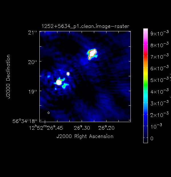
Important: A key indicator for any self-calibration that is going correctly is to observe the increase in $\mathrm{S/N}$ per iteration. DO NOT rely on just measuring the rms as the self-calibration model could be bad and is artificially reducing all amplitudes!
2. Inspect model (step 2)
Let's Fourier Transform this model that you've generated back into the measurement set. This will generate model visibilities that will be used as a guide for self-calibration solutions.
ft(vis='***',
   model='***', # remember to use the new model!
   usescratch=True)
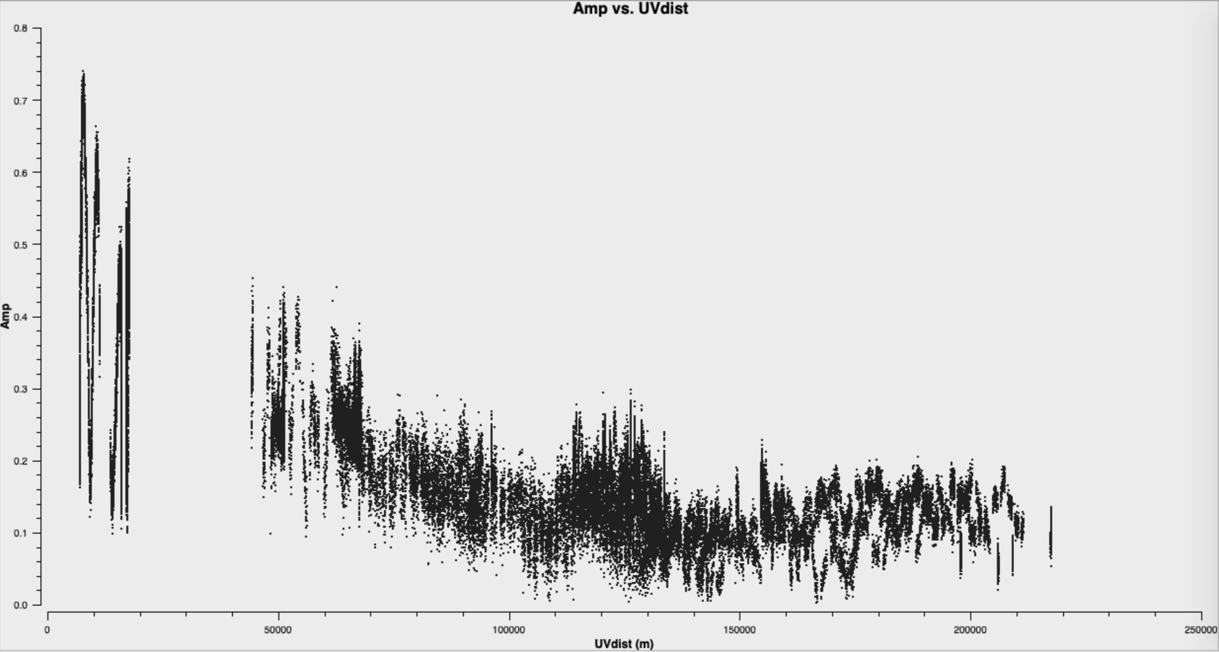
The second part of this step will plot the model and amplitude against $uv$ distance for just spw 0. Using the interactive plotms module, adjust the y axis to add the $\texttt{DATA}$ column to see how the model fits to the data. For more information on how to do this refer to the CASAdocs documentation for plotms. You can also adjust it to data-model (by changing the ydatacolumn parameter) to observe the discrepancies between the model image and the observed visibilities. Note that only one spw is plotted for speed.
plotms(vis=target+'_E19.ms',
 		   xaxis='uvdist',
 		   yaxis='amp',
 		   spw='0',
 		   ydatacolumn='model',
 		   correlation='RR,LL',
 		   avgchannel='64',
 		   coloraxis='spw',
 		   plotfile='3C277.1_uvdist_modelp1.png',
  		   overwrite=True)
Here is $uv$ distance versus amplitude
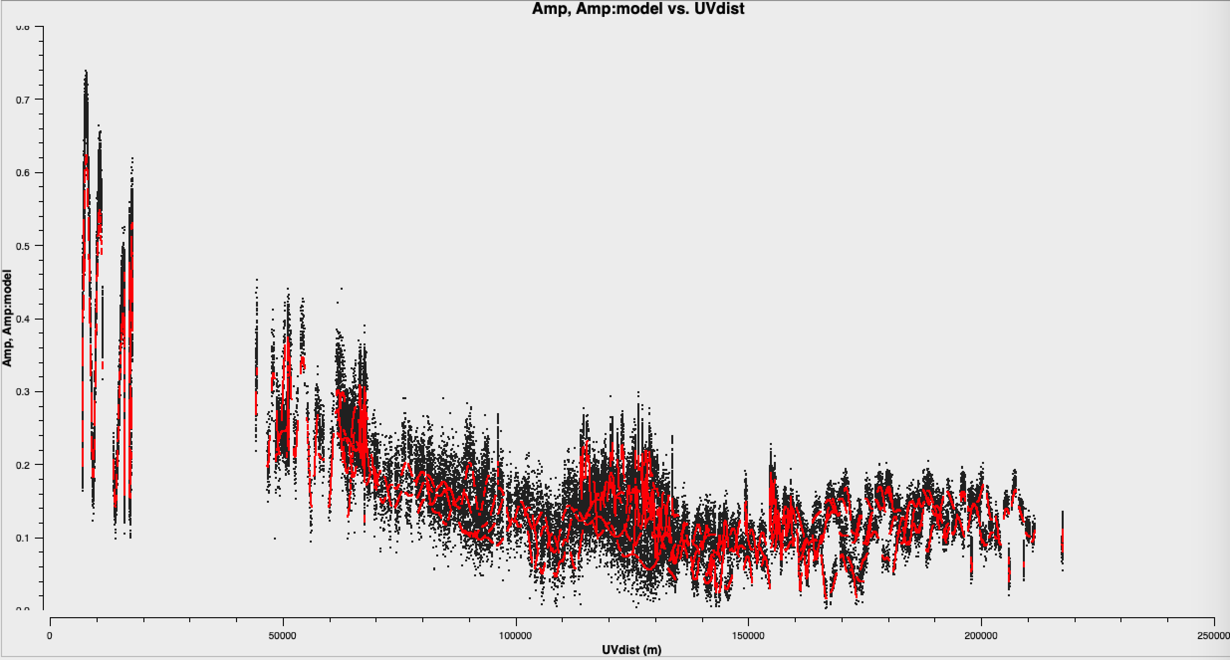
And with the model column overlaid (by going to Axes, Add Y axis and then change the Column tab within the interactive plotms GUI)
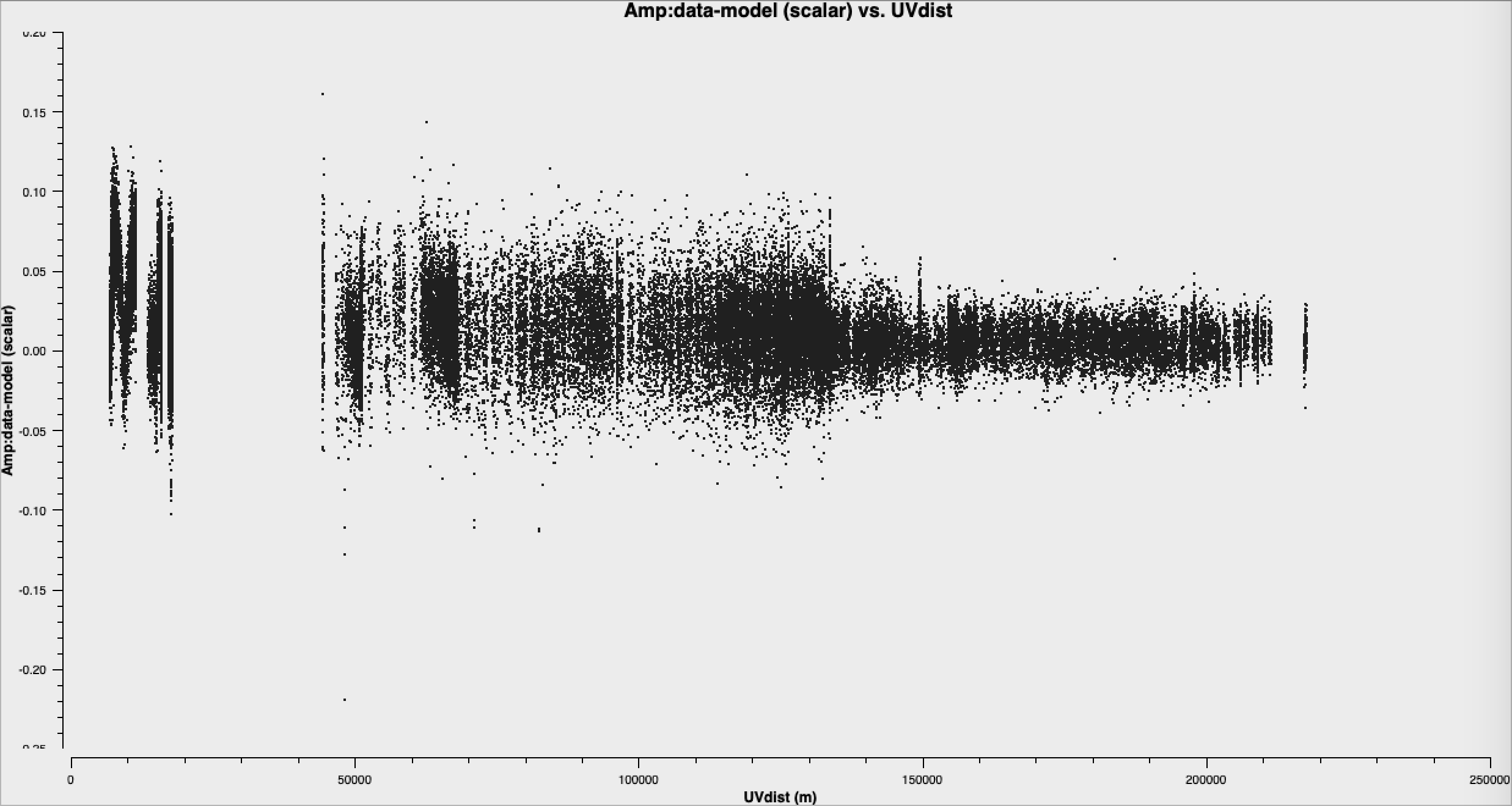
And for the data-model column, see that the residuals are mis-calibrated data + noise:
3. Inspect to choose interval for initial phase self-calibration (step 3)
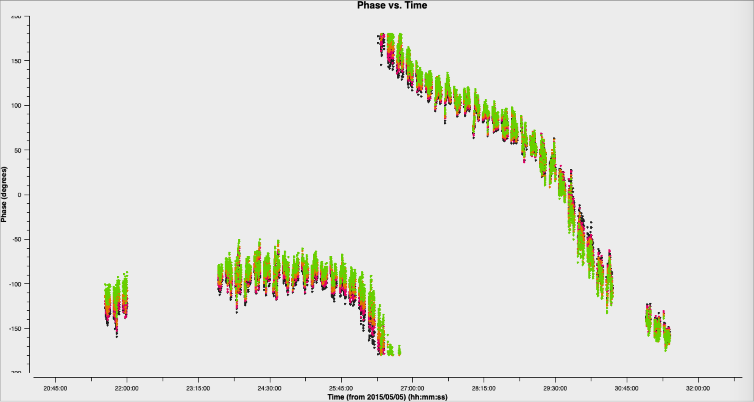
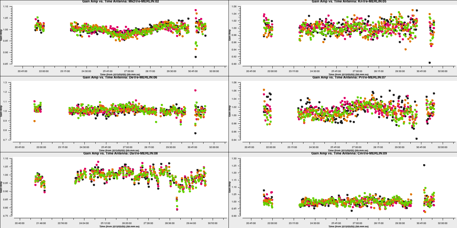
It is hard to tell the difference between phase errors and source structure in the visibilities, but it helps to balance between choosing a longer interval to optimise S/N, and too long an interval (if possible the phase changes by less than a few tens of degrees). The phase will change most slowly due to source structure on the shortest baseline, Mk2&Pi, but you should also check that the longest baselines (to Cm) to ensure that there is enough S/N. Plot phase against time, averaging all channels per spw (see listobs for the number of channels).
plotms(vis='***'',
	   xaxis='***',
	   yaxis='***',
	   antenna='***',
	   correlation='***',
	   avgchannel='**',
	   coloraxis='spw',
	   plotfile='',
	   overwrite=True)
The first plot shows the long timescale phase changes that illustrates the source structure and the bottom plot shows a zoom on a few scans that illustrate the faster phase fluctuations induce by the atmosphere. The chosen solution interval should also ideally fit an integral number of times into each scan.
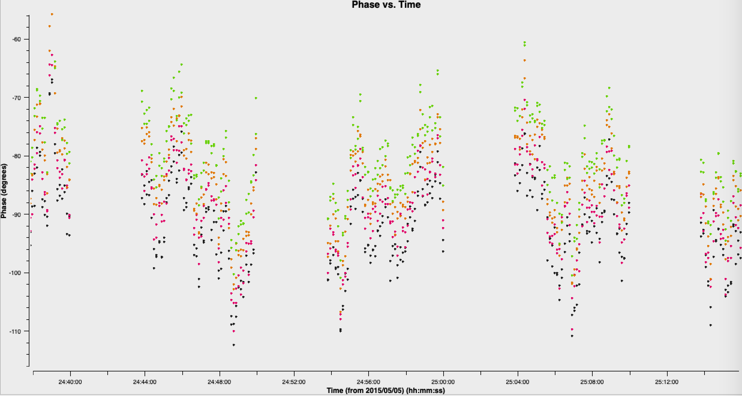
As we have a pretty strong model (SN$>$200), let's use a short solution interval. Heuristics suggest that 30s is usually about the shortest worth using, because the atmosphere is reasonably stable on these baseline lengths at this frequency.
4. Phase-self-calibrate again (step 4)
Run gaincal, with solint to 30s and write a new solution table (the new model will be used). We only want to do a phase only solution remember!
os.system('rm -rf target.p2')
gaincal(vis='1252+5634.ms',
calmode='***',
caltable='target.p2',
field=target,
solint='***',
refant='Mk2', ## from imaging!
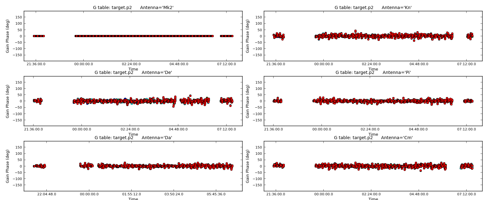
minblperant=2,minsnr=2)Plot the solutions.
5. Apply the solutions and re-image (step 5)
Use default applycal parameters, but just adding the gaintable as the calibration solutions you just created.
applycal(vis='1252+5634.ms',
		 gaintable='***')
From listobs, the total bandwidth is almost 10% of the frequency, which is enough to take the spectral index into account. Cotton et al. (2006) finds a spectral index varies from -0.1 in the core to as steep as -1.
listobs shows that the total bandwidth is 4817 to 5329 MHz, i.e. for flux density $S$, $S_{4817}/S_{5329} = (4817/5329)^{-1}$ or about 10%. The improved S/N gives much greater accuracy. Thus, in order to image properly and produce an accurate image to amplitude self-calibrate all spectral windows, multi-term multi-frequency synthesis (MT-MFS) imaging is used. This solves for the sky model changing across frequency.
Make sure you clean till as much target flux as possible has been removed into the model - you can increase the number of iterations interactively if you want.
tclean(vis='1252+5634.ms',
	   imagename='1252+5634_p2.clean',
	   cell='***arcsec',
	   niter=1000, # stop before this if residuals reach noise
	   imsize='***',
	   deconvolver='mtmfs',
	   nterms=2, # Make spectral index image w/ linear fit
	   interactive=True)
Use ls to see the names of the image files created. The image name is 1252+5634_p2.clean.image.tt0.
If we check the image using the same boxes as before (just use the same imstat commands as in Step 2 but change the imagename!), I get $S_p \sim 171.360 \,\mathrm{mJy\,beam^{-1}}$ and $\sigma \sim 0.443\,\mathrm{mJy\,beam^{-1}}$. This is another large $\mathrm{S/N}$ increase to $\sim 387$.
Let's put the model we derived into the visibilities. To encode the frequency dependence of the source we need to include both terms of the model (i.e. the tt0 and tt1 models).
ft(vis='1252+5634.ms',
   model=['***.model.tt0','***.model.tt1'], # model images from the MTMFS images,
   nterms='**', # same as tclean!
   usescratch=True)
6. Choose solution interval for amplitude self-calibration (step 6)
Plot amplitude against time in order to choose a suitable solution interval.
plotms(vis='1252+5634.ms',
	   xaxis='***',
	   yaxis='***',
	   ydatacolumn='***',
	   antenna='Mk2&**',
	   correlation='**,**',
	   avgchannel='**',
	   coloraxis='spw')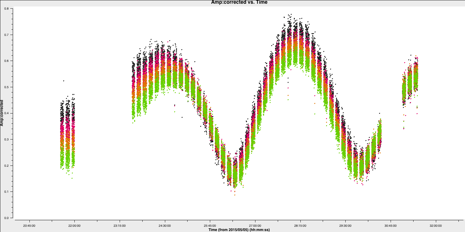
The amplitudes change more slowly than phase errors and a suitable solint is a few times longer than for phase.
7. Amplitude self-cal (step 7)
In gaincal, the previous gaintable with short-interval phase solutions will be applied, to allow a longer solution (averaging) interval foramplitudee self-calibration. Set up gaincal to calibrate amplitude and phase, with a longer solution interval, and the same refant etc. as before.
os.system('rm -rf target.ap1')
gaincal(vis='1252+5634.ms',
		calmode='***',              # amp and phase
		caltable='target.ap1',
		field='1252+5634',
		solint='***',
		refant='Mk2',
		gaintable='***',  # the phase table should be applied
		minblperant=2,minsnr=2)
Plot the solutions. They should mostly be within about 20% of unity. A few very low points implies some bad data (high points). If the solutions are consistently much greater than unity then the model is missing flux.
8. Apply amplitude and phase solutions and image again (step 8)
Use applycal to apply the short-interval phase solution table and the amplitude and phase table you have just created.
applycal(vis=target+'.ms',
		 gaintable=['**','**'])
Clean the image again, as before and inspect.
tclean(vis='1252+5634.ms',
	   imagename='1252+5634_ap1.clean',
	   cell='***arcsec',
	   niter=1500, # stop before this if residuals reach noise
	   imsize='***',
	   deconvolver='mtmfs',
	   nterms='**', # Make spectral index image
	   interactive=True)
Again, with the same boxes, I get $S_p \sim 171.717 \,\mathrm{mJy\,beam^{-1}}$ and $\sigma \sim 0.174\,\mathrm{mJy\,beam^{-1}}$. This now corresponds a huge $\mathrm{S/N}\sim 987$. The key message with self-calibration is to increase the S/N of your observations by removing calibration errors whilst not constraining your visibilities to the model. Due to the number of free parameters, you need to use an iterative approach to obtain the true source structure! It takes practice to know what's right and wrong.
9. Reweigh the data according to sensitivity (step 9)
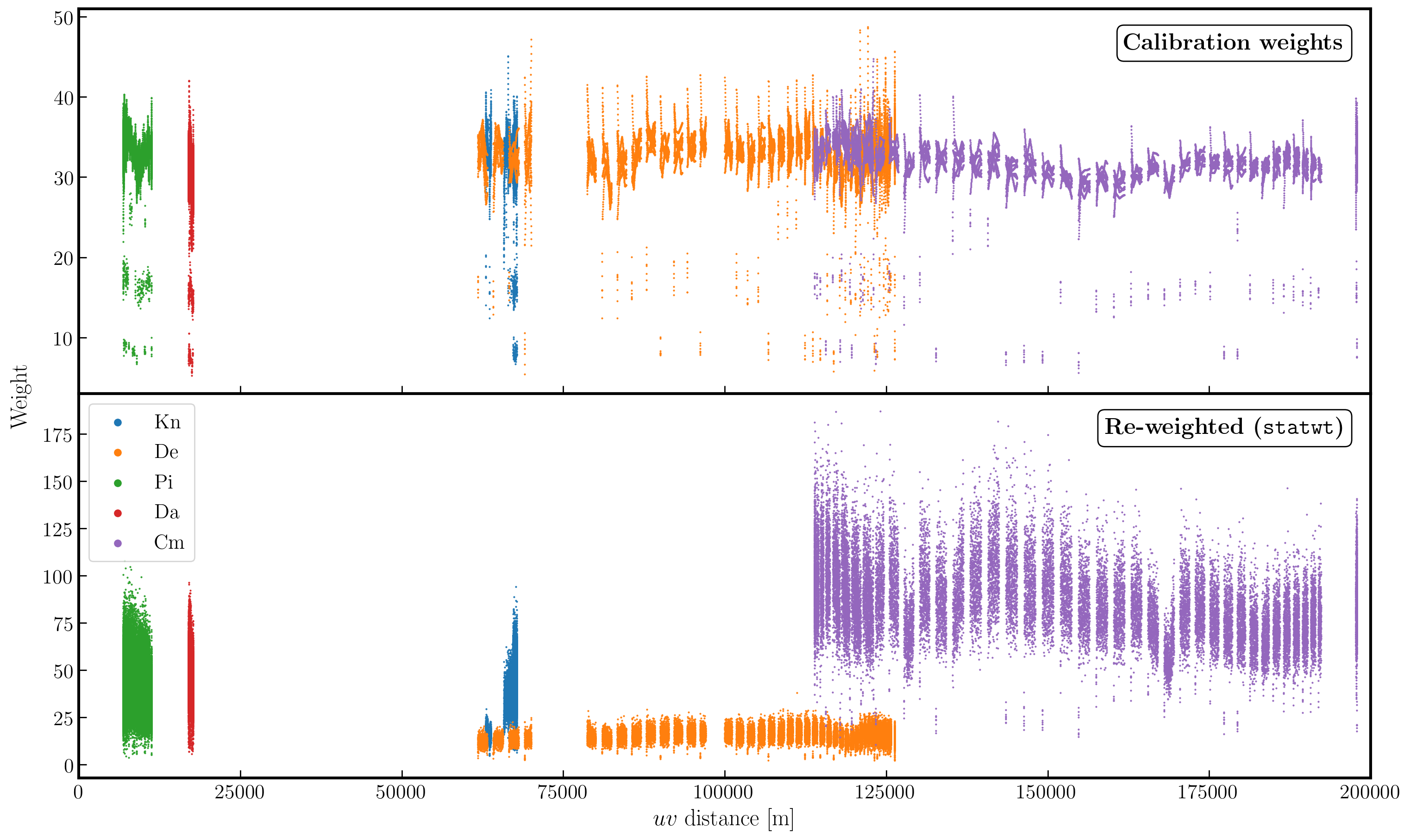
Often, especially for heterogeneous arrays, the assigned weighting is not optimal for sensitivity. For example, the Cambridge (Cm) telescope is more sensitive, therefore, to get the optimal image must be given a larger weight than the other arrays.
To recalculate the optimal weights we use the task statwt calculates the weights based on the scatter in small samples of data. Note that the original data are overwritten, so you might want to copy the MS to a different name or directory first.
There are alot of options here, but we are just going to use the default options. You can try with different weightings if you'd like.
statwt(vis='***')
In the plot below, we show the weights before (top panel) and after re-weighting (bottom panel) on the baselines to our refant (Mk2). As you can see, the telescopes have similar weights despite Cm being more sensitive. With the use of statwt, the weights now reflect the sensitivities, and have also adjusted some errant weights which were low before.
10. Final image & multi-scale CLEAN (step 10)
Let's image the re-weighted data using multiscale clean, which instead assumes that the sky can be represented by a bunch of Gaussians rather than delta functions. Have a look at the help for tclean, which suggests suitable values of the multiscale parameter.
tclean(vis='1252+5634.ms',
	   imagename='1252+5634_ap1_multi.clean',
	   cell='***arcsec',
	   niter='***', # stop before this if residuals reach noise
	   imsize='***',
	   deconvolver='***', # find the multiscale option (mtmfs does it!)
	   scales=['**','**','**'], # add scales to use (in pixels)
	   nterms='*', # also want mtmfs!
	   interactive=True)
You will find that the beam is now slightly smaller (I got $60\times44\,\mathrm{mas}$) as the longer baselines have more weight, so the peak is lower. I got $S_p \sim 151.086 \,\mathrm{mJy\,beam^{-1}}$ and $\sigma \sim 0.076\,\mathrm{mJy\,beam^{-1}}$.
11. Summary and conclusions
We began with a simple phase-reference calibrated data set of our target. Here, the phase and amplitude corrections are valid for our nearby phase calibrator, but crucially only approximately valid for our target. This is because the patch of sky the telescopes are looking through for the target, is not the same as the phase calibrator.
For our target source, the assumption that our source is a simple point source in invalid (as proven by the uv distance plots). This means that, in order to calibrate for the gain differences between the phase cal and target fields, we need to produce a model to calibrate against. The approximate phase and amplitude solutions are just valid enough for us to derive a first order model.
Once we generated a model using deconvolution, the Fourier Transform of these are used to calibrate against. We begin with phase only calibration as this needs less S/N for good solutions. With these corrections applied, we can generate a much better model whose S/N has increased dramatically. This S/N boost can then be used to then calibrate for amplitudes and phases. As a result, we end up with a high dynamic range data set (with a high S/N), where lots of low level source structure has appeared. The following table and plot illustrates this vast improvement.
| Peak Brightness | Noise (r.m.s.) | S/N | |
|---|---|---|---|
| [$\mathrm{mJy\,beam^{-1}}$] | [$\mathrm{mJy\,beam^{-1}}$] | ||
| Phase referencing | 151.925 | 1.896 | 80.129 |
| Phase self-calibration (cycle 1) | 169.130 | 0.807 | 209.579 |
| Phase self-calibration (cycle 2) | 171.360 | 0.443 | 386.817 |
| Amp+phase self-calibration | 171.717 | 0.174 | 986.879 |
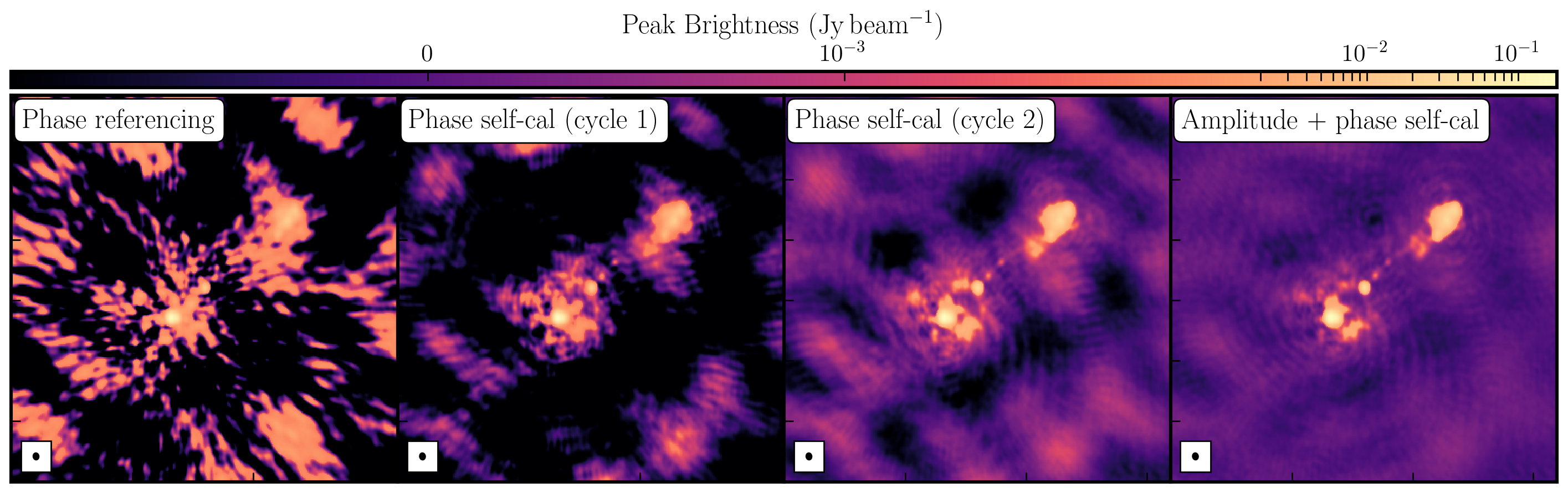
In this tutorial, we fixed residual calibration errors associated with approximate gain and phase solutions derived from the phase calibrator, the second part investigated the various imaging techniques which can be used to extenuate features. In the first instance we used statwt to optimally reweigh the data to have maximum sensitivity. We find that the Cm telescope is the most sensitive (as it is 32m wide), but also contains all the long baselines. As a result these long baselines are expressed more when imaging resulting in a higher resolution image than what we've seen before. As a result the peak flux reduces but so did the sensitivity! In addition, we used multiscale clean to better deconvolve the large fluffy structures which standard clean can struggle with.