Supplementary Material to:
An Introduction to Radio Astronomy
4th edition Cambridge University Press 2019
Last updated 10/08/2019
Prologue
The radio signal from source to
reception – a brief recapitulation
·
Starting
points
o
The challenge of radio astronomy is to
measure tiny amounts of power in random noise signals from natural sources in
the face of (much larger) unwanted sources of noise, typically from the
receiver itself but also from other “stray” radiation entering the system.
o
Radio Frequency Interference (RFI)
produced by humans can be millions of times stronger than natural noise
signals.
o Disregarding RFI, only
integrated noise powers (the Stokes parameters) are observable at a single
point in space.
o Differential
phase can be measured at two points (with an interferometer).
o
In the classical Rayleigh-Jeans regime
(![]() )
the power emitted by a black body (BB) per unit bandwidth is directly
proportional to its physical temperature T (K). The specific intensity (units
W m-2 Hz-1 sterad-1; see
also below) is
)
the power emitted by a black body (BB) per unit bandwidth is directly
proportional to its physical temperature T (K). The specific intensity (units
W m-2 Hz-1 sterad-1; see
also below) is
![]()
o Most
sources are not BBs but it is convenient to assign to them the equivalent brightness
temperature of a BB emitting the same specific intensity. This route also gives
rise to the concepts of antenna temperature and system noise temperature. They
are convenient ways to characterize power spectral density (per Hz) or power
(over a finite bandwidth).
o Quantum
effects become important at the point where the BB spectrum (the Planck
equation) deviates from the linear Rayleigh-Jeans approximation: the latter is
applicable at frequencies (in GHz)
well below ~20T.
o
Radio photons have very low energies and quantum statistical effects can
be ignored up to THz frequencies. Radio waves can be therefore be amplified and
manipulated in complex receiving systems without loss of information.
·
The
brightness of a source and its flux density
o At emission
the intensity of a source at a given frequency is called the specific
intensity (![]() with units W m-2 Hz-1 sterad-1); the observed
specific brightness (
with units W m-2 Hz-1 sterad-1); the observed
specific brightness (![]() also with units W m-2 Hz-1
sterad-1) is identical only if
the entire antenna beam is filled with radiation at the source temperature; off-axis
“sidelobes” usually pick up radiation from different temperature material. The
equality also breaks down due to absorption (using the equation of radiative
transfer; see below), scattering of radiation out of the line of sight and
cosmological redshift.
also with units W m-2 Hz-1
sterad-1) is identical only if
the entire antenna beam is filled with radiation at the source temperature; off-axis
“sidelobes” usually pick up radiation from different temperature material. The
equality also breaks down due to absorption (using the equation of radiative
transfer; see below), scattering of radiation out of the line of sight and
cosmological redshift.
o The
specific intensity is set by source physics not
by the distance; the inverse square law is a solid angle effect and as a
discrete source moves away it gets smaller not less “bright”.
o A
good approximation to the true source brightness can be obtained if the source
is larger than the beam – but the measurement is always subject to errors
due to uncalibrated pick-up through the sidelobes.
o An
approximation to the source brightness can be obtained via the beam dilution
method if the source size is comparable to the beam size (see the example in
Supp. Mat Chapter 5)
o The
source brightness is not accessible if the source is much smaller than beam; in
this case can only obtain the more limited quantity – the flux density (units W
m-2 Hz-1) which is the brightness integrated over the
beam.
· Radio sources emit
random noise from a variety of processes: (see also Supp. Mat. Chapter 2 )
o Thermal radiation (unpolarized
at emission)
- black body: from terrestrial
objects, planetary surfaces, interstellar dust, the cosmic microwave background
- free-free or bremsstrahlung:
from ionized plasmas
- atomic and molecular
lines: from many species in the ISM and molecular clouds
o Non-thermal (usually polarized)
- synchrotron:
from the ISM, supernova remnants; active galaxies
- molecular masers:
from comets; stellar atmospheres; evolved stars; star
forming regions and active galaxies.
- coherent radiation:
from solar bursts; pulsars, fast radio burst sources.
·
The ionized plasma in the Interstellar Medium (ISM) modifies the
received radiation:
o Absorption at lower
frequencies by the free-free process – diagnostic of the square of the electron
column density along the line of sight.
o Dispersion (pulsars
and bursts) with higher frequencies arriving first (see also Supp.Mat Chapter 15) – diagnostic of the electron column
density in the ISM plasma along the line of sight.
o Faraday Rotation of the
plane of linear polarization (see also Supp. Mat Chapter 4) due to the
difference in propagation speeds of the hands of circular polarization in a
magnetized plasma – diagnostic of magnetic fields along the line of sight.
o Scintillation and
scattering (much stronger at lower frequencies; see also Supp Mat Chapter 4) –
diagnostic of small scale density irregularities.
·
The Earth’s ionospheric
magnetized plasma modifies the received radiation at low frequencies
o Does
not allow propagation below the plasma frequency - typically ~10 MHz but highly
variable with time of day and solar activity.
o Imparts differential
phase delays across an array hence disturbs the complex visibility function at
frequencies up to ~2 GHz.
o Imparts
Faraday Rotation which can be significant up to ~2 GHz.
·
The Earth’s neutral atmosphere modifies the received radiation
at high frequencies
o Emits additional
thermal noise and attenuates the signal (application of the equation of
radiative transfer; see below). Clear-sky opacity:
- Is dominated by water
vapour (proportional to the precipitable water vapour PWV) and oxygen absorption.
- reduces
with altitude: statistically falls exponentially with scale height (~2km for
water; 8.5 km for oxygen)
- is time
variable: water vapour is poorly mixed and over a
given site varies unpredictably with wind strength and direction
- rises
with zenith angle (za) : proportional to sec(za)
·
The equation of radiative transfer (Rayleigh
Jeans regime)
o Commonest
case used in radioastronomy is a background source
seen through a semi-transparent cloud in Local Thermodynamic Equilibrium
![]()
where ![]() is the optical depth (i.e. opacity per unit length x distance).
is the optical depth (i.e. opacity per unit length x distance).
· The antenna and its characteristics
o The
antenna couples the incident radiation field to the receiver system producing a
fluctuating voltage (zero mean); this voltage can be manipulated in the
electronics with the output being the average power measured within
particular frequency bands.
o At
frequencies of a few hundred MHz and below various forms of wire antenna are
most cost effective; at higher frequencies parabolic antennas dominate.
o In a
parabolic antenna the energy flow is via the “feed” at one of the foci; the signal power collected
from a given source per unit time depends on:
- The geometrical
collecting area of the antenna Ageom and its aperture
efficiency yielding the effective area Aeff.
- The main factors
which affect Aeff are:
1. blockage
from the primary focus cabin or secondary mirror and their support structures
2. surface
imperfections and hence reflectivity calculated with the Ruze
formula
3. the
illumination taper towards the aperture’s edge – choice depends on the
importance of sidelobe levels for the application.
- The receiver
bandwidth ![]()
o The Antenna
Temperature TA is defined as the temperature of a matched resistor imagined
to be heated by the collected radiation. A resistor acts like a 1-D black body
and the maximum power available is kT![]() (watts). If the reception pattern is filled
with emission of brightness temperature TB then TA = TB ; the system is acting like a radio
thermometer or “radiometer”.
(watts). If the reception pattern is filled
with emission of brightness temperature TB then TA = TB ; the system is acting like a radio
thermometer or “radiometer”.
o The power beam
pattern is the Fourier Transform of the Autocorrelation Function (ACF) of the
aperture distribution (an application of the Wiener-Khinchin
Theorem).
o The antenna
equation
![]()
is a fundamental relationship for a given
aperture; the antenna beam solid angle ![]() refers
to the power collected over
refers
to the power collected over ![]() steradians including the main lobes and the
sidelobes.
steradians including the main lobes and the
sidelobes.
o The width of the main lobe depends on the illumination taper but
typically the full width at half maximum (FWHM) ~ 1.2 λ /D radians where D is
the antenna diameter.
- N.B. this is NOT an approximation to 1.22 λ
/D which is the radius of the
1st null in the “Airy disk” i.e. the beam produced by uniform illumination
of a
circular
aperture.
- More
gradual taper (greater power collected from the edge of the dish) produces
higher sidelobes but a smaller main beam width and thus higher Aeff; sharper
taper produces the opposite effects.
o The antenna beam convolves (smooths) the true
sky brightness distribution which can be imagined as a grid of closely-spaced
(<< beamwidth) points; discrete sources
separated by less than one FWHM are hard to discern as distinct objects.
o Equivalently the
antenna response weights the angular frequency Fourier components (cycles per
radian) which describe the sky by an angular frequency transfer function
(i.e. the
ACF of the aperture distribution). The ACF therefore acts like a low-pass filter weighting
and eventually cutting off the sky’s angular frequency spectrum.
o To
map the sky and avoid aliasing data are taken at angles separated by less than
half the FWHM (effectively the Nyquist criterion); in practice data are taken at
3 points per FWHM.
o For a point source observing a source of flux density S:
![]()
![]() acts as a useful indicator of
antenna performance in terms of K/Jy; some values from
which to scale: a dish of diameter 25m and aperture efficiency 56% produces an
antenna temperature rise of 0.1K/Jy.
acts as a useful indicator of
antenna performance in terms of K/Jy; some values from
which to scale: a dish of diameter 25m and aperture efficiency 56% produces an
antenna temperature rise of 0.1K/Jy.
o The antenna pointing
needs to be accurate to <0.1 FWHM in order that power variations during
tracking are less than a few percent.
· The receiver
o Since
the incident power is very small the receiver chain must provide high amplification
(typically >100 dB) before natural signals can be measured and quantified.
o
Noise powers add: since
sources of input radiation are incoherent the antenna temperature TA is the
sum of the independent noise temperatures e.g.
![]()
o Loss before the first amplifier (e.g. due to an anti-RFI filter) both attenuates the received signal and adds noise to it
![]()
where ![]() is the transmission coefficient and Tatten is the physical
temperature of the attenuator. This is a
simplified
version of the equation of radiative transfer for high transmission (small attenuation). The effect of the signal loss on the overall signal-to-noise ratio can be described
as an unattenuated signal with a further-enhanced system noise level.
is the transmission coefficient and Tatten is the physical
temperature of the attenuator. This is a
simplified
version of the equation of radiative transfer for high transmission (small attenuation). The effect of the signal loss on the overall signal-to-noise ratio can be described
as an unattenuated signal with a further-enhanced system noise level.
o An amplifier generates
self-noise as if there was a resistor of temperature TLNA at its
input. At deci- and centimetric wavelegnths
TLNA is typically <50K at room temperature and
<5K if the amplifier is cryogenically cooled to <20K.
o Tracing power flowing through a receiver: with several stages each producing different
noise temperatures T and with power gains G yields an equation for the
receiver temperature:
![]()
If the first stage gain G1 ~ 30
dB or more then Tsys ~ T1 and one
can effectively ignore all other noise contributions from the rest of the
stages – even if some are just lossy (like mixers) since their noise is
“swamped”. N.B. loss before the first
amplifier cannot be recovered.
o Mixers have conversion loss: typically at
least 6dB (i.e. a factor 4); this can be treated as a “gain” < 1 i.e. Gmixer~ 0.25 when tracing power through a
receiver.
o System noise budgets: depend
on
- whether the receiver is cryogenically cooled;
- pick-up from sidelobes;
- frequency (lower frequencies “see” more of the Galaxy; higher
frequencies suffer more from atmospheric noise)
- altitude (to reduce the atmospheric contribution);
- At λ = 21cm (1420 MHz) an excellent cryo-cooled receiver has Tsys ~ 20 K (~45K uncooled); at λ = 1cm (30 GHz) an good cryo-cooled
receiver has Tsys ~ 40 K (sea-level). In space the cryo-cooled Planck spacecraft LFI
receivers (30 and 44 GHz) had Tsys ~ 10K since only TLNA + TCMBR contribute.
- For a summary of international radio telescope and receiver performance
see the review by Bolli et al (2019) https://arxiv.org/abs/1907.02491
o A
single signal channel is only sensitive to one orthogonal component of
polarization – polarization measurements require two channels. They can be
linear [X,Y] or circular [L,R] pairs; appropriate combinations
of either pair yield the 4 Stokes power parameters I,Q,U,V.
o Temperature
calibration is carried out with respect to two or more temperature sources at
known physical temperatures using the Y-factor method. Passive temperature controlled loads or active noise sources at a
previously calibrated equivalent temperatures can be used. If the two temperatures are widely separated
then care must be taken to ensure that the receiver output is linear (or a
third temperature comparison source used).
o The
radiometer equation yields the maximum signal-to-noise ratio achievable for a
given system temperature Tsys; bandwidth ![]() and integration time
and integration time ![]() .
.
![]()
o
Extreme receiver gain
stability is often required in order to be able to integrate for long enough to
detect very weak natural emission in the face of the system noise. Such stability is usually not available due
to changes in temperature (slow), variations in power supply voltages (all
timescales); quantum effects in the LNA transistors (rapid) etc. These lead to
fractional gain variations ![]() ~ 10-4 to 10-5 on
integration times of interest.
~ 10-4 to 10-5 on
integration times of interest.
o
Gain variations (“1/f noise”) typically increase linearly with time t hence with 1/f where f is the
frequency of the output fluctuations (not the RF frequency); they are
independent of thermal noise so the two effects add quadratically giving a
total rms
![]() ]1/2
]1/2
o
The “knee frequency” or
integration time (1/fknee) is when ![]() i.e when
i.e when ![]()
-
In the case of cryo-cooled high bandwidth
systems e.g. the Planck LFI receivers the thermal noise is very low and fknee can be
as high as ~100 Hz i.e. gain variations dominate the fluctuations on timescales t > 10 millisec.
The correlation receiver architecture (see Supp. Mat. Chapter 6) increased this
by about three orders of magnitude
o
For total power systems the
effect of gain variations can be much reduced by switching against or
correlating with a reference signal .
-
Dicke-switch receiver:
(see also Supp. Mat. Chapter 6) compares the gain-fluctuating
output against a reference load. BUT since the antenna is only connected to the
source ½ the time and two noisy signals are being differenced the radiometer
equation becomes:
-
Twin-beam receiver: (See also
the OCRA-p system in Supp Mat Chapters 6 & 8) Dicke-switched
receivers have only one beam looking at the target and do not compensate for
variations in atmospheric transmission and variations in stray radiation
(mainly ground spillover). By using a twin-beam system one can mitigate gain variations
and also eliminate a large fraction of the atmospheric variations since in the
near field the cylindrical reception patterns (approximately the diameter of
the antenna) largely overlap. Since one of the beams is always observing the
source the radiometer equation becomes:
- In the far-field the beams do not overlap. If the source is compact, and
falls in only in one beam, it is seen in the difference. BUT an extended source
produces similar signals in each beam and the difference tends to zero – the
receiver can be said to be “differentiating the sky”.
o Heterodyne receivers:
it can be easier and cheaper to amplify, filter and
generally manipulate signals at lower frequencies than the observing frequency.
- Other advantages
i) helps to avoid the danger of
oscillation if all the ~100dB of gain is at the same frequency; ii) minimises loss in signal transport cables; allows the centre frequency under study to be easily changed by varying the LO
frequency.
- Non-linear mixers (see illustration in Supp. Mat. Chapter 6) are used to
create cross-products of the signal with a fixed frequency Local Oscillator (LO);
the basic action can be visualised as a continuous
on-off switch - the conductance of a diode is controlled by
the varying local oscillator (LO) voltage.
The output contains a wide range of harmonics of LO and RF and mixture
products. Both sum and difference frequencies are also generated but commonly one selects the difference
frequency; the other sideband is usually filtered to prevent “out of band”
signals contaminating the observing band.
- Linear transformation: after
the mixing and filtering processes the relative
amplitudes and phases of the input frequency components are preserved despite
the use of non-linear circuit elements. This is vital for interferometry.
· Polarisation
o Polarisation
measurements provide information about the emission region and the propagation
path to the observer:
- synchrotron sources, pulsars/FRBs and masers are intrinsically polarised but polarisation
can be induced in unpolarised emission during
propagation e.g. by scattering.
o Radio astronomy receivers ideally respond to two equal magnitude
orthogonal electric field components: either two linears
or two circulars;
- linear polarisation can be translated to
circular by means of a 90o relative phase shift (equivalent to a
“quarter wave plate” in optics) and vice versa.
o
The practical definition of
RH and LH circular polarization in radio astronomy are those radiated away
from RH and LH helical antennas (i.e. as seen from source). For RH (LH) circular
the tip of the E-vector rotates anti-clockwise (clockwise) as seen from the
observer.
o
Stokes Parameters: I
(total intensity), Q (linear),U (linear) ,V(circular)
are practical, measurable, power quantities. Partially polarised
radiation is described by linear combinations of powers measured in orthogonal
directions; there are several formulations (see Chapter 7).
o Natural noise sources require averaging < > to smooth out
fluctuations:
Linearly polarized flux density p =
(<Q2> +
<U2>)1/2
Fractional linear polarisation: p/I =
(<Q2> + <U2>)1/2/ I
Position angle of linear polarisation ![]() = ½ tan-1[<U>/<Q>]
= ½ tan-1[<U>/<Q>]
Complex polarization ![]() = Q +iU
= Q +iU
o Measuring Stokes parameters: can be done with orthogonal linear or
circular receiver channels – each has advantages and disadvantages and each is
widely used. Circular is demanded in VLBI while it is typically easier to
achieve broad bandwidths with linear receivers.
· Signal digitisation (see also Appendix 3)
o
Amplitude
-
For pure random noise one can use
single bit digitization (above or below zero mean) with only loss of 36% (the van
Vleck formula) in signal-to-noise ratio; but with
zero mean single bit digitization is not useful for total power radiometry.
-
Multi-bit digitization is needed
for radiometry and for subtraction of RFI; up to 14 bits are now used for
precision subtraction.
o
Time/frequency
-
Nyquist-Shannon theorem: an analogue signal
containing no frequencies higher than ![]() can be reconstructed
exactly by sampling that function at a frequency (rate) of at least
can be reconstructed
exactly by sampling that function at a frequency (rate) of at least ![]() . Any frequencies above the Nyquist frequency
are “aliassed” i.e. folded back into the band.
. Any frequencies above the Nyquist frequency
are “aliassed” i.e. folded back into the band.
·
Signal processing
concepts (see also Supp. Mat Appendix 1)
o
Convolution: is a smoothing operation relating an input to an output
through a linear system response, equivalently using:
- functions in time, space or angle: the output is the convolution with the system’s
“impulse response” function; analytically one of the functions is flipped
around before step-wise integration.
OR
-
temporal
spatial or angular spectra: (Fourier components): the system’s complex
“Transfer Function” reweights the components of the input spectrum to give the
output spectrum; both amplitudes and phases but not the frequencies, of the
output Fourier components are altered.
o
Correlation: is equivalent to multiplication and
integration:
-
Autocorrelation: measures the similarity of a function at different delays compared
with the undelayed version hence picks out periodicities but loses signal phase
information.
-
Wiener-Khinchin Theorem: FT [ACF] = power spectrum of signal (or
vice versa with inverse FT)
-
Cross-correlation: measures
similarities between independent signals - preserves phase information and most
used in synthesis interferometry.
· Spectrometry
o
Digital
Autocorrelation Spectrometers
(DACS) and Fast Fourier Transform Spectrometers (FFTS) correspond
to different sides of the Wiener-Khinchin theorem.
o DACS (described in Section 7.2 and 7.3 and Supp. Mat Chapter 7) require
specialised digital logic and are now being superseded by FFTS. Commonality with commercial
requirements means that FFTS can use “off-the-shelf” high-speed integrated circuits
(high speed ADCs + Field Programmable Gate Arrays FPGAs).
·
Interferometers: delay and fringe spacing
o the critical parameter in all interferometry is the geometrical time delay
τg = b.s/c (seconds) where b is the baseline vector (metres) between two
antennas and s is the unit vector pointing towards the source; with![]() defined as the angle between the
direction perpendicular to the baseline and the source direction τg = b sin
defined as the angle between the
direction perpendicular to the baseline and the source direction τg = b sin ![]() /c. To achieve coherence the parts of the wavefront striking each antenna must be brought together
with τg having been compensated electronically;
/c. To achieve coherence the parts of the wavefront striking each antenna must be brought together
with τg having been compensated electronically;
o the projected baseline is that component measured perpendicular
to the source direction = b cos ![]() (metres)
or = b cos
(metres)
or = b cos ![]() (wavelengths); for small angles
away from the pointing direction the fringe period = λ/b cos
(wavelengths); for small angles
away from the pointing direction the fringe period = λ/b cos ![]() (radians) and the corresponding
angular fringe frequency = b cos
(radians) and the corresponding
angular fringe frequency = b cos ![]() (cycles per radian); the primary
antenna beam pattern provides an overall envelope to the quasi-sinusoidal “fringe
pattern”.
(cycles per radian); the primary
antenna beam pattern provides an overall envelope to the quasi-sinusoidal “fringe
pattern”.
· Adding interferometers (direct imaging):
o can be imagined as parts of the surface of a dish but with
electrical delays, rather the paraboloidal shape of the reflecting surface, bringing
the voltage signals together in phase.
o
the antennas, receivers and
associated electronics convert the incoming electric field to voltages,
preserving their relative amplitudes and phases (as above); the outputs are
added together and then square-law detected and an instantaneous power beam is formed
(see Supp. Mat. Chapter 8) just as for a dish – hence this is direct imaging
and forms the basis of phased arrays (see Supp. Mat. Chapter 8 and end of Supp.
Mat Chapter 11).
o
In addition to the
interference term dependent on the geometrical delay the output power has positive
offset terms due to antenna temperatures and, mainly, receiver noises.
·
Multiplying
or correlation interferometers (indirect imaging):
o the total
power terms disappear by multiplying and integrating the signals leaving only
the interference term with zero mean.
o for a discrete source the interferometer responds to a locally cosinusoidal fringe pattern on the sky; it effectively multiplies the source
brightness distribution by this pattern and
integrates the result over the source to form one Fourier component of the brightness
distribution. Each observation with a
given baseline length and orientation provides a new Fourier component.
o Cosine (Rc) and sine (Rs)
channels (correlated with a λ/4 difference in delay) are required to describe
asymmetric brightness distributions (see below); the complex visibility
function (i.e. a complex Fourier component) is defined as:
![]() with
amplitude A = (R2c
+ R2s)1/2 and phase
with
amplitude A = (R2c
+ R2s)1/2 and phase ![]() = tan-1 (Rs/Rc)
= tan-1 (Rs/Rc)
o the phase is measured in terms of the local fringe period in radians and
represents the position of that Fourier component
with
respect to a fiducial position in the source
o if the variable delay is tracked perfectly the moving source remains at
the same place relative to the fringe patterns – this implies perfect knowledge of
the baseline geometry &
source position and no propagation effects.
o phase shift
equivalences
-
change the time delay τg by travel
time of one RF cycle and the position of the fringe pattern moves by one fringe
spacing (cycle).
-
change the assumed source position on the sky by
one fringe spacing (or cycle) and the interferometer output changes by one
cycle
-
propagation delay variations have major impacts on
astrometric/geodetic position measurements and, via the corresponding phase
shifts, the alignment
of Fourier components for imaging
o
the observed visibility data require further
processing to produce the image – hence this is indirect imaging.
·
Temporal (longitudinal)
coherence and the interferometer “delay beam” :
o An interferometer
measures the coherence of wave trains at two points. The temporal coherence (how statistically similar is a function to a delayed
copy) is measured along the direction of propagation and is codified in the
Wiener-Kinchin Theorem. Away
from the pointing angle the additional delay produces a decorrelation which reduces
the measured visibility. A first order estimate yields a requirement on
the allowed field-of-view:
![]()
i.e.
the inverse of the fractional bandwidth of the frequency channel times the
fringe spacing (with b being
the baseline in wavelengths); to avoid this limitation the band
is split into many narrow frequency channels.
· Spatial (transverse) coherence and the interferometer visibility function :
o interferometers
measure the degree of spatial or
lateral coherence (the correlation) of the wavefront
transverse to its direction of propagation.
o emission regions are sums of incoherent point sources; each contributes
to the combined electric field at each antenna in a baseline giving some degree of correlation
between them. When the baseline is larger the differential delays become
significant and the combined fields at the separate antennas become
increasingly dissimilar – the degree of lateral coherence reduces and hence the
interferometer response falls
- the source is “resolved”.
o The van Cittert-Zenicke Theorem: the mutual
correlation function in space is the Fourier Transform of the brightness
distribution of the source. The Visibility Function is another name for the
spatial correlation function.
·
Synthesis image
construction: the
visibility data from N(N-1)/2 baselines are the (sampled) complex visibility
function; the final image is constructed from the inverse Fourier transform of
these data. Unless the relative phases
have been measured accurately, a distorted image results.
Even if the phases are perfectly known the imperfect sampling and lack of
sensitivity to the total power within the field-of-view produces fluctuations
and negative regions in the constructed image.
o
The (u,v) plane:
u,v are the E-W and N-S (some authors swap these around) components of the baseline
vector in wavelengths. The u,v
plane sampling is built up using many (sometimes relocated) antennas plus Earth rotation. A source at the celestial
pole produces circular tracks over 24h, at other positions tracks are ellipses
(incomplete when source sets).
o Hermitian symmetry: the sky
brightness distribution is real i.e. it is a 2-D array of scalars (simple
numbers).
- The FT of a real function has definite symmetry; the FT of an even
(symmetric) function is also even (the cosine transform); the FT of an odd (antisymmetric)
function is also odd (the sine transform).
Hence V(u,v) =
V*(-u,-v) implying
that the visibility measured on a baseline from antenna 2 to antenna 1 is
predictable from that measured on 1 to 2 (the phase is reversed). Hermitian points are always added into the u,v plane to ensure that the
inverse transform producing the “Dirty Beam” and the “Dirty Map”, will be real.
o The “Dirty Beam” or point spread function (psf)
is the FT of the (u,v)
coverage with unity flux at the sampled points; the “Dirty Map” is the FT of
the sampled visibility function V(u,v)
o Imperfect u,v sampling (missing/unmeasured
Fourier components): there are an infinite number of brightness distributions compatible with
the sampled V(u,v); the Dirty Map (sometimes called the
“Principal Solution”) is just the one
with V(u,v) = 0 at the unsampled points (clearly a non-physical assumption). In
addition to the inevitable limitation on resolution due to a finite maximum baseline, specific distortions due to missing Fourier
components are:
- reduced sensitivity to low brightness structure and insensitivity to the
total power in image from inadequate coverage of short spacings
- negative regions – which cannot be physically correct since sky is
positive;
- complicated sidelobe structure in general which confuses the science
interpretation.
o The “Dirty Map” is the convolution of the true sky with the “Dirty Beam”:
one cannot “deconvolve” the data in the u,v (i.e. Fourier) plane by classic linear image
processing methods i.e. by reweighting the data with the inverse of the
transfer function (the u,v coverage) since the
transfer function contains zeros and so the inverse would “blow up” – the problem
is said to be “ill-posed”.
o Non-linear deconvolution: the
answer is to work in the sky (i.e. image) plane albeit the aim of any
algorithm must be to generate new, plausible, visibility data (complex Fourier
components) to “fill in the u,v gaps” - more realistic
images will then be produced. The algorithm should enforce sky positivity and can
include different assumptions about the sky’s statistical properties. The most
commonly used method is the CLEAN algorithm (Section 10.9) which is based
on the assumption that the sky can be approximated by a set of point
sources. Even the first point source
makes predictions about the visibility function in unmeasured regions since the
Fourier Transform of a point source extends out to infinity with a baseline
dependent phase variation depending on its position. Many improvements have
been made to the original algorithm.
·
Correlation interferometer
sensitivities:
o
Point-source:
-
the rms flux density close to that of a single antenna whose area equals
the total effective area of the sum of the interferometer antennas.
o Brightness temperature:
- the rms temperature limit is the radiometer equation multiplied by 1/(array
filling factor) but this relation can be optimistic if the u,v
coverage of short baselines is poor.
“Discovery
Space”
Astronomers are constantly striving to discover
and describe new phenomena in the Universe.
The track record of the radio astronomy community is outstanding (see Chapter 1) and it
is worthwhile being aware of the lessons of history.
· Classically (e.g. Harwit, M., 1981, Cosmic Discovery; Harwit, M., 2003, Physics Today, 56, 38) “astronomical discovery space” (in any waveband) involves significant improvements enabled by technical innovation in one or more of:
o sensitivity;
o angular resolution;
o sky coverage;
o temporal coverage (from nanoseconds to years);
o spectral coverage and resolution.
· The above constitute the classical axes of “observational phase space” but new “meta-axes” are coming into play in radio astronomy
o high speed digitization, manipulation and storage;
o machine learning and AI to extract information from big (real-time and archived) data sets
· Never forget that it is people who make the discoveries, hence the more eyes and brains focused on the data the better; this is the “human bandwidth” meta-axis described by Wilkinson (2007, 2015). Two basic means of maximizing the human bandwidth are:
o the ability to re-examine archived data;
o “commensal observing”, encouraged by the increasing fields-of-view of radio telescopes, where more than one group gains access to the incoming data.
· Two final points:
o There is no all-encompassing approach to radio telescope design; dishes and arrays have complementary roles and there is new science waiting at all resolutions and wavelengths.
o Radio telescopes are rarely known for the astronomical goals which led to their construction !
Further reading:
·
“Serendipitous Discoveries in Radio
Astronomy” proc. NRAO Workshop Green Bank
W.Va. 1984 eds. K.I. Kellerman and
B. Sheets http://library.nrao.edu/public/collection/02000000000280.pdf
·
J. Cordes et al. “Discovery and understanding with the SKA”, SKA Memo 85 (2006)
·
Ekers R.D. ”Big
and Small” Paper
presented at Special Session 5, IAU General Assembly XXVII, Rio de Janerio,
August 11, 2009.
https://pos.sissa.it/099/007/pdf
· Kellerman
K.I. et
al “The Exploration of the
Unknown” Paper presented at Special Session 5,
IAU General Assembly XXVII,
Rio de Janerio, August 11, 2009. https://pos.sissa.it/099/005/pdf
·
Norris, R. P. 2017. “Discovering the
Unexpected in Astronomical Survey Data”. PASA,
34(Jan.), e007. See https://arxiv.org/abs/1611.05570
·
Norris, R. P. 2017. “Extragalactic radio
continuum surveys and the transformation of radio astronomy”, Nature Astronomy, 1(Oct.), 671–678. See https://arxiv.org/abs/1709.05064
·
Wilkinson, P. N., Kellermann,
K. I., Ekers, R. D., Cordes, J. M., and W. Lazio, T.
J. 2004. “The exploration of the unknown”. New
Astron. Rev., 48(Dec.), 1551–1563. https://arxiv.org/abs/astro-ph/0410225
·
Wilkinson, P.N. 2007 “Exploration of
the Unknown” in From Planets to Dark
Energy - The Modern Radio Universe https://pos.sissa.it/052/144/pdf
·
Wilkinson, P.N. 2015 “The SKA and the
Unknown Unknowns” in Advancing
Astrophysics with the Square Kilometer Array (editor SKA Organisation) https://pos.sissa.it/215/065/pdf
The philosophy and practicalities
of “discovery” in astronomy continue to generate ideas: as witness the
following “White Papers” submitted to the US 2020 Decadal Survey
·
Bellm, E. et al., “ Scheduling Discovery in the 2020s” https://arxiv.org/abs/1907.07817
·
Fabbiano G., et al., “Increasing the Discovery
Space in Astrophysics” https://arxiv.org/abs/1903.06634
·
Hickish, J. et al. “Commensal
Multi-user Observations with an Ethernet-based Jansky Very Large Array” https://arxiv.org/abs/1907.05263
·
Najita, J. “Investing for Discovery in Astronomy” https://arxiv.org/abs/1907.11700
Chapter 1: The Role of Radio Observations in
Astronomy
Radio observation bands – complement
to Figure 1.1
|
Band |
Characteristic
wavelength |
Frequency
|
Best to observe from |
|
sub-mm
wave |
100
microns |
3 x
1012 Hz (3
THz) |
aircraft,
balloons, space |
|
millimetre-
wave |
1 mm
|
3 x
1011 Hz (300
GHz) |
mountains,
balloons, space |
|
centimetre-wave
|
1 cm |
3 x
1010 Hz (30
GHz) |
mountains,
surface in good weather |
|
metre-wave |
1 m |
3 x
108 Hz (300
MHz) |
ground
|
|
decametre-wave
|
10 m
|
3 x
107 Hz (30
MHz) |
ground
|
|
hectometer-wave |
100 m |
3 x 10⁶ Hz (3 MHz) |
space |
Early Radio Astronomy –
historic telescopes
To illustrate Chapter 1 of IRA4 we present a series of key
events and discoveries up to 1969, starting with Jansky.
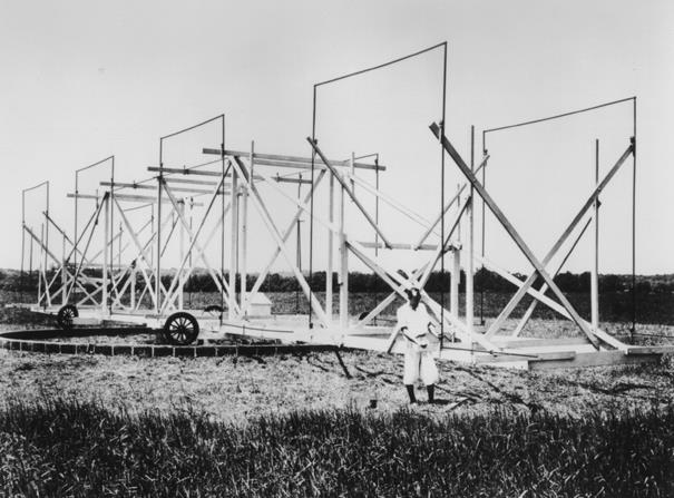
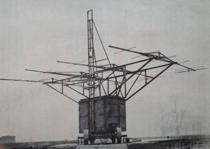
1933 Karl Jansky, working at Bell Labs identified the source of background radio noise as extraterrestrial and associated with the Milky Way galaxy. He used this steerable antenna at 15 metre wavelength (20 MHz).
1940 Grote Reber constructed the first parabolic reflector radio telescope single-handedly in his garden. Using it he produced a map of galactic radio emission at 160 MHz.
1946 Stanley Hey and co-workers mapped the Northern sky at 64 MHz with an array of four Yagi antennas situated near London, UK. They drew attention to a intense discrete radio source in the constellation of Cygnus (later named Cygnus A) which showed strong fluctuations.
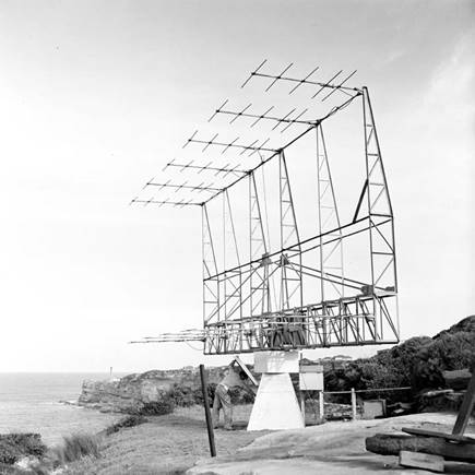
1948 John Bolton and co-workers used a series of cliff-top interferometers in Australia and New Zealand better to locate Cygnus A and discover other discrete sources
including Taurus A, Virgo A and Centaurus A
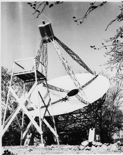
1950 The first radio source identified beyond the Milky Way. Robert Hanbury Brown and Cyril Hazard discovered radio emission from M31, the Andromeda Nebula, using the 218 ft parabolic reflector at Jodrell Bank. The surface was made out of poles and wires with the focal point able to be moved to track a source by tipping the central support pole. Its final incarnation (around 1959) is shown in the right hand image (see also https://www.flickr.com/photos/30974264@N02/5031194415/in/album-72157624924398355/). The larger central support tower has been tipped over to provide access to the focus from a fixed platform. (colour image courtesy of Wayne Young).
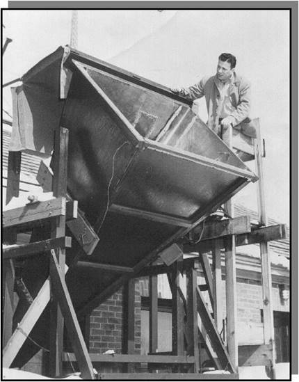
1951 The hydrogen line at 21 cm wavelength Harold Ewen and Edward Purcell made the ground-breaking discovery at Harvard University, using this horn antenna. Other groups in Australia and The Netherlands soon followed.
1954 The radio galaxy Cygnus A was optically identified based on a position obtained by Graham Smith (seen here) with an interferometer consisting of two Wurzberg reflectors in Cambridge..
1950s Surveys of radio sources. The 2C (and subsequently 3C and 4C) interferometers. Large numbers of radio sources were discovered by Martin Ryle an co-workers in Cambridge, using interferometers with parabolic cylinder reflectors and by Bernard Mills and co-workers in Australia using the Mills Cross (below).
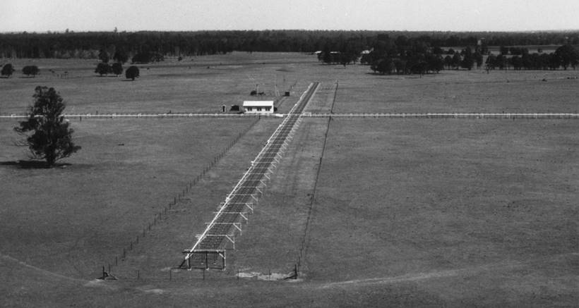
1954 Surveys of radio sources. The original Mills Cross, built at Fleurs, NSW, Australia with EW and NS arms 450 m long, at 3.5 m wavelength.
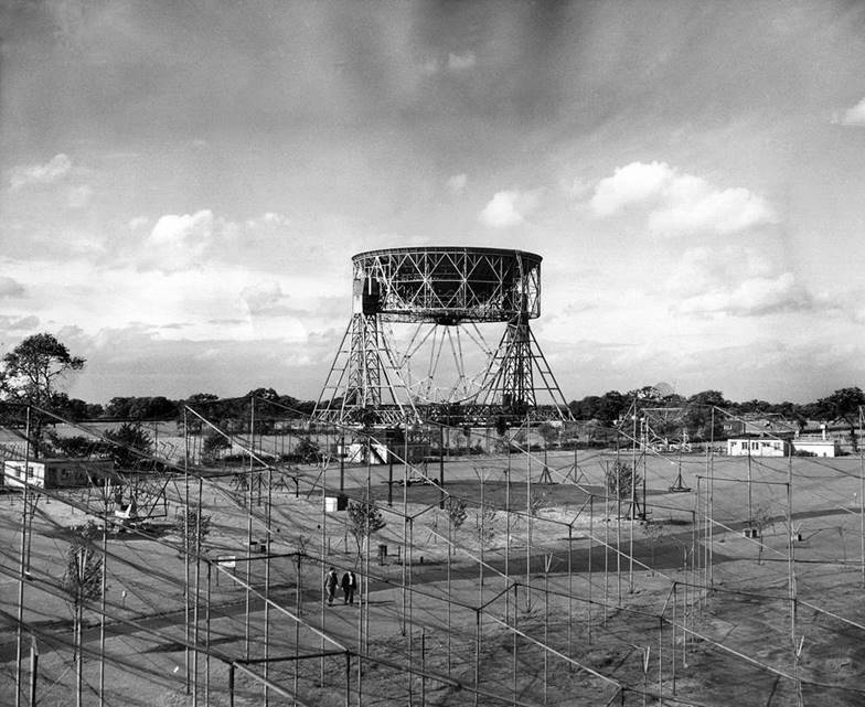
1957 The University of Manchester’s Jodrell Bank Mk1 telescope: The world’s first “giant” fully-steerable paraboloid with a diameter of 250 feet (76 m) was built under the direction of Bernard Lovell. In the foreground is its precursor the 218ft telescope (as above). In its early years the Mk1 played a significant role in tracking/commanding US and Soviet spacecraft.
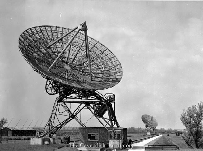
1962 Developing interferometer techniques led to the One-Mile Telescope at Cambridge which, under Martin Ryle and Anthony Hewish, “broke open” the technique of aperture synthesis imaging.
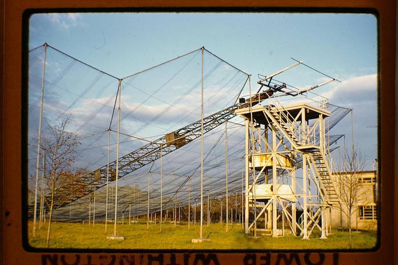
1963 First detection of molecules by radio. Absorption lines at 18 cm wavelength from the hydroxyl radical were discovered by Sandy Weinreb and co-workers (Nature 200, 829) using the 84-ft. parabolic antenna of the Millstone Hill Observatory of the MIT Lincoln Laboratory coupled with Weinreb’s digital autocorrelation spectrometer.
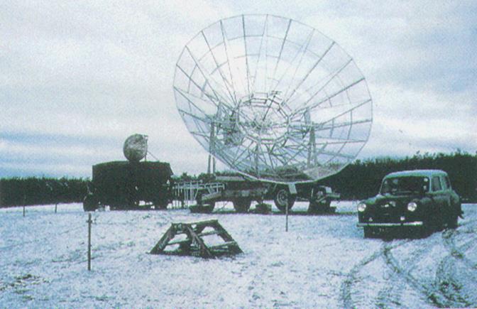
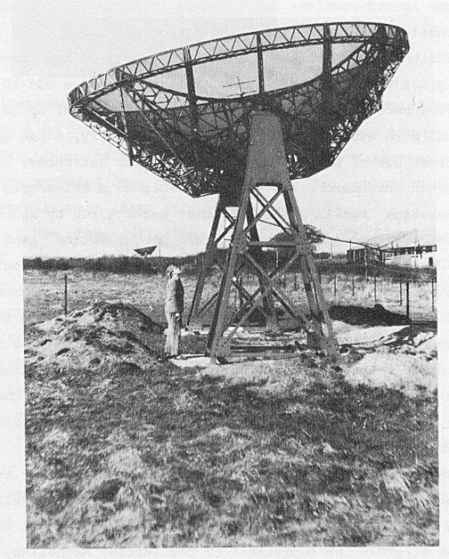
Early 1960s: Development of real-time long baseline interferometry in Manchester. Here a portable steerable 25-ft paraboloid has been radio-linked with the Mk1 telescope at Jodrell Bank (see above) over a baseline of 131 km. The bright compact radio sources revealed on such baselines were an important factor in the discovery of quasars.
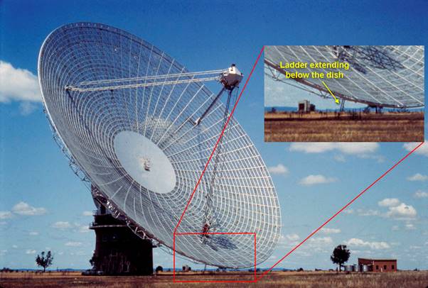
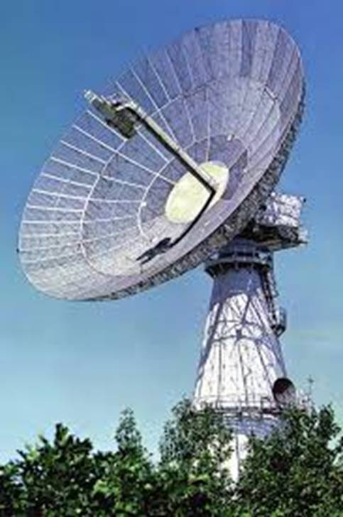
1963 The identification of 3C273 – the first quasar. Cyril Hazard and co-workers used the 210 ft Parkes telescope in Australia to establish an accurate position for the bright compact radio source 3C273; soon afterwards Maarten Schmidt established a redshift z=0.158 for the faint stellar optical identification: see the story at https://www.parkes.atnf.csiro.au/people/sar049/3C273/
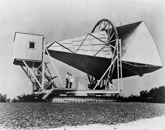
1965 The Cosmic Microwave Background was discovered by Arno Penzias and Robert Wilson, using a ‘sugar-scoop’ horn at Bell Labs in Holmdel New Jersey. The low sidelobe level of the horn enabled accurate (to ~1K) absolute power levels to be established - a new era of cosmology had begun.
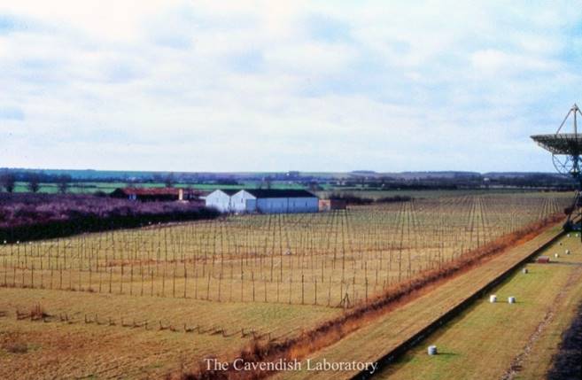
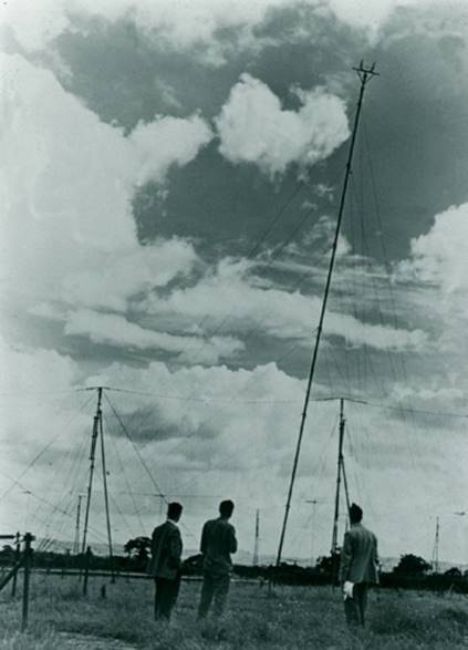
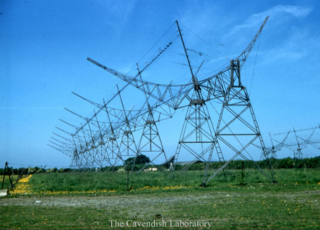
1967 Pulsars were discovered at Cambridge University by Jocelyn Bell and Antony Hewish, using a large array of dipoles at 3.7 m wavelength.
Additional references for the history
of radio astronomy
In addition to the references in the text and in Further Reading we also recommend the following, each of which presents the developments from a different perspective.
·
The Origins of Radio Astronomy in: http://www.jb.man.ac.uk/distance/exploring/course/content/module1/
· Birth of Radio Astronomy: Chapter 3 in “Radio Telescope Reflectors” by J.W.M. Baars and H.J. Kärcher, Astrophysics and Space Science Library No 447, (2017) pub. Springer https://link.springer.com/content/pdf/10.1007%2F978-3-319-65148-4.pdf
· The Development of Radio Astronomy: R. Wielebinski and T. Wilson, Chapter 13 in Portal to the Heritage of Astronomy (IAU) https://www3.astronomicalheritage.net/index.php/show-theme?idtheme=18
·
The History of Jodrell Bank http://www.jb.man.ac.uk/history/
· A Brief History of
Radio Astronomy in Cambridge https://www.astro.phy.cam.ac.uk/about/history
·
The
beginnings of Australian radio astronomy, W.T. Sullivan,
Journal of Astronomical History and Heritage ,
Vol. 8, p. 11-32 (2005).
·
“But it was Fun: the first forty years of radio
astronomy at Green Bank” eds F.J. Lockman, F.D. Ghigo &
D.S. Balser,
Pub. National Radio Astronomy Observatory (2007) ISBN 10: 0970041128 , ISBN 13: 9780970041128. See
also http://www.gb.nrao.edu/~fghigo/biwf/biwf2/biwf2016final7opt.pdf