The Origins of Radio Astronomy
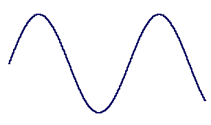
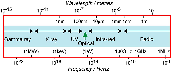
The Electromagnetic SpectrumRadio waves are electromagnetic radiation just like the visible light to which our eyes are sensitive and just like the X-rays which we use in medical imaging. Each consists of an electric and magnetic wave which oscillate together just like waves on a stretched string, Figure 1. The only difference between these various forms of electromagnetic (EM) radiation is their wavelength i.e. the distance between consecutive peaks (or troughs). Gamma-rays have the shortest wavelength and radio waves the longest, see Figure 2. These type of waves are called transverse waves in which the up and down path shown in Figure 1 actually represents the variation with time (the increase and decrease) of some property such as, in this case, the electric or magnetic field strengths. If you were to stand at some point in space as an EM wave travelled past you would measure the electric field increase and then decrease repeatedly. The number of complete cycles which you feel each second is called the frequency of the wave. This is measured in cycles per second, now referred to as Hertz (after the physicist who first transmitted radio waves in the laboratory in 1888). Obviously, the frequency and the wavelength are related by the speed at which the wave travels. This is expressed in the formula
where c is the speed of light in a vacuum in metres per second,
Obviously the earliest astronomical observations were made in the visible part of the spectrum. However it is now possible to make observations across the whole range of wavelengths. Indeed it is essential to adopt a multi-wavelength approach in order to improve our understanding of the wider universe. In this course we shall see what a thorough study of the radio part of the spectrum has enabled us to determine about the nature of the universe and we shall look at some of the techniques by which we detect and analyse radio emissions. The American PioneersAs with many of the most exciting discoveries in astronomy, the first observation of radio waves from outer space was by chance. An American radio engineer, Karl Jansky, born in Oklahoma, and a graduate of Wisconsin University, joined the Bell Telephone Laboratories in New Jersey and was assigned the task of dealing with the problems being suffered by short wave radio telephone links due to interference. One major problem with the reception of overseas telephone reception was that of crackling static noises and, in order to attempt to discover their origin, he built a large directional antenna, operating at a wavelength of 14.6m, which could be moved to look towards the horizon in any direction. One hundred feet in length, the antenna, shown in Figure 3, rotated on a set of four Ford Model T car wheels!
Jansky was able to show that the cause of the static crashes was lightning. He recorded the effects of both local thunderstorms and also those from more distant ones reflected from the ionosphere. But he also became aware of a more subtle form of interference - a gentle hissing noise similar to the background noise produced by the radio receiver itself. (Note: much effort has gone on since then to reduce this receiver noise to an absolute minimum.) At first Jansky thought that the Sun might be the source of the noise, but, following a year of careful measurements, he realised that, instead, it appeared to come from a specific region of the sky.
This conclusion came from the fact that, if he kept his antenna pointing due south, the weak signal reached a peak every 23 hours and 56 minutes. This is the period of a sidereal day - the time kept by the Earth with respect to the stars - and is less than the solar day
(24 hours) by 4 minutes due to the fact that the Earth, as well as rotating about its own axis is also in orbit around the Sun. This adds to the effective rotation rate with respect to the stars and so the sidereal day is less - see Figure 4. He found that the peak of his signal occurred when the telescope was pointing towards the constellation Sagittarius - towards the centre of our galaxy, the Milky Way!
Jansky, pictured in Figure 5, had thus discovered that celestial bodies could emit radio waves as well as light waves. He suggested that the origin of this radiation might be ionised interstellar gas rather than stars but it was a long time before its true origin was found. So, at the age of 26, Jansky, has made an historic discovery, but his results, published in 1932, received little attention and it was not until the late 1940's that the significance of his achievements was widely appreciated. He suggested that a parabolic antenna should be constructed to provide more precise observations but there was no support for his proposal and, as we shall see, it was left to an amateur radio astronomer to continue his work. Sadly, he died in 1950 at the young age of 44, so was not able to see the rapid growth of a new field of astronomy in the 1950's and 60's. Radio astronomers do honour his achievement however, as the unit of radio flux (the strength of the received radio waves) is called the Jansky. A full size operational replica of his antenna has been built at Green Bank, West Virginia, the home of the world's largest fully steerable radio telescope. It was built by the same carpenter who had worked on the original! The original antenna had been removed sometime in the 1950's. Recently, a number of old photographs of the Jansky antenna were found which enabled its precise location at Holmdale to be found, and a memorial consisting of a 13ft model of his antenna has been sited there.
Jansky's work was continued by a second American radio engineer called Grote Reber pictured in Figure 6. Born in Chicago in 1911, he graduated in 1933 and worked for a number of radio manufacturers during the period 1933 to 1947. He became interested in the science of radio astronomy when he read one of Jansky's articles and determined to continue it. During just 4 months in 1937 he built the world's first dedicated radio telescope in his backyard at Wheaton, Illinois - a 31 ft parabolic antenna, also shown in Figure 6, that could be moved to point to any part of the sky. The sheet metal reflector focused the radio waves to a point 20ft above the surface where an amplifier located within the cylinder amplified the very weak signals by many millions of times so enabling the strength of the signals to be plotted on a chart. The tower to the left of the dish enabled Reber to gain access to the receiver.
Reber initially attempted to use the relatively short wavelengths of 9 and 33cm since, as we shall see below, these would give his telescope better imaging quality than at longer wavelengths, but without result. He then tried a wavelength of 1.9m (160 MHz) and finally, in 1938, was able to confirm Jansky's observations, Figure 7. Interference from car ignitions systems was a problem and he was forced to observe at night! This success encouraged him to build a better receiver with which he was eventually able to detect the Sun and also a strong radio source in the direction of the constellation Cassiopea. Now known as Cassiopea A (the A indicating the strongest source in that constellation), this was the first discrete radio source to be detected outside our solar system, but it was many years before its true nature was discovered. Reber presented his surveys of the sky as contour maps which showed the arc of the Milky Way as bright areas. As Jansky had shown, the brightest area corresponds to the centre of the Galaxy in the direction of Sagittarius, see Figure 8. His results from the period 1938 to 1943 were published in both engineering and astronomy journals and ensured that radio astronomy became a major field of research after the war. In the early 1960's Reber donated his telescope to the National Radio Astronomy Observatory (NRAO) at Green Bank where he also supervised the construction of the replica of Jansky's antenna referred to above.
Non-Thermal RadiationReber's observations showed that some other mechanism than normal "thermal emission" must be responsible for the radio emission that he was observing. Thermal emission is the name given to emission, stretching across the whole electromagnetic spectrum, from any body which radiates simply because it is hot. This is why we can see the Sun since, at a temperature of 6000K, it is radiating strongly in the visible part of the spectrum. But it also radiates in the radio part of the spectrum, though with far less energy. Thermal emission is also called "Black Body Radiation" and has a precise form discovered by Max Planck as he developed Quantum Theory in the early years of the Twentieth Century. There are two empirical laws that relate to the nature of the emitted power in blackbody radiation. Stefan's Law states that the total energy emitted increases as the 4th power of the temperature, whilst Wien's Law states that the wavelength of the peak of the emission is inversely proportional to the temperature (so hotter bodies emit most of their energy at shorter wavelengths than colder ones). Thus all objects above absolute zero in temperature will radiate across all parts of the electromagnetic spectrum and thus produce some radio emission. The Moon, for example, is also visible in the radio. With thermal radiation in the radio regime, as one observes at higher frequencies the signal strength would be expected to increase but Reber found that, instead, the signals were weaker. He realised that some other "non-thermal" process must be at work. The problem was resolved by a Russian physicist, V.L. Ginsburg, who showed that electrons moving at speeds close to that of light (termed relativistic electrons) in the magnetic field of the galaxy would be forced to move along a path similar to a helix in form. Part of the motion of the electron is thus circular - i.e., it goes round a circular path as it also moves forwards - this implies that the electrons must be being accelerated and, when accelerated, electrons will radiate. This radiation is called Synchrotron Radiation as it was discovered experimentally when the first synchrotrons - circular devices in which electrons are accelerated round a circular track defined by a ring of magnets - were built. The galaxy is full of relativistic electrons and other particles blasted into space by the explosions of massive stars (supernovae). (When they enter the Earth's atmosphere these high-energy particles are known as Cosmic Rays.) We believe that such electrons, spiralling through the magnetic field of the Galaxy, give rise to the radiation observed by Jansky and Reber and, as Reber found, the power from this type of radiation does decrease at higher frequencies. One advantage of using a much shorter wavelength than Jansky was that the angular resolution (sharpness) of Reber's observations was nearly three times better. (~14 degrees i.e. the smallest structures one can map out have angular scales of about 14 degrees, the Full Moon has an angular diameter of 0.5 degrees - see below). A reasonably detailed map of the radio sky could thus be made and showed that the majority of the radiation came from the galactic plane (the plane of the Milky Way), with a maximum towards the galactic centre. It also showed two "hotspots" of radiation in the constellations of Cygnus and Cassiopeia. One of these was, in fact, the first indication of strong radio sources well beyond our own galaxy.
NOTE: The resolution of an antennaReber used a 31 ft, 9.4m, diameter antenna at a wavelength of 1.9m. We will explain in detail how such an antenna works and why it is restricted to receiving radiation from a small region of the sky called its beamwidth in a later module. For the moment, accept that the laws of physical optics can be used to estimate the beamwidth of a circular antenna. The classical formula is:
Where
You should be able to show that for Reber's antenna described above this gives a
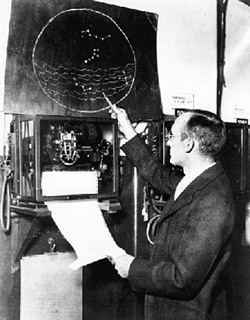
value for Wartime DevelopmentsNot surprisingly, during World War II, little was done to extend the work of Jansky and Reber, though the technology of radio and radar advanced greatly. As we shall discuss further in the next module, in February 1942 severe interference jammed the British early-warning radar systems and it was shown that their source was within a few degrees of the Sun. J.S Hey, observing these reports concluded that the interference was probably associated with a large sunspot group that was crossing the disc of the Sun - the beginnings of solar radio astronomy. Radar systems also sometimes suffered from transient echoes. Hey's work showed that they came from ionized meteor trails. The energy of the dust particle passing through the Earths upper atmosphere strips the outer electrons away from their nuclei and so they become free to oscillate in sympathy with a radio wave falling on them. The electrons are thus being accelerated and will radiate themselves, so producing an echo. (It is the presence of free electrons within a metal that renders them suitable for making the reflecting surfaces of radio antennas.) Here was the beginning of "radar astronomy". Hey was also able to show that the enhanced radio noise coming from the constellations Cygnus and Cassiopeia were due to two intense discrete sources of radio waves rather than general areas of the sky.
The war years also produced a highly significant theoretical breakthrough which lead to the development of a major field of Radio Astronomy. A copy of Grote Reber's paper in The Astrophysical Journal reached the Leiden Observatory in Holland, then under Nazi occupation. Jan Oort, its Director, realised that, should any of the
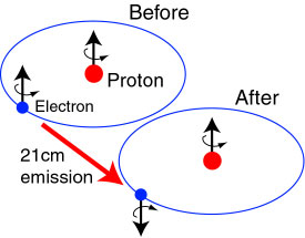
atoms or molecules in space give rise to a spectral line in the radio part of the spectrum, it would enable much information about the interstellar medium to be found. For example, the relative velocity of a gas cloud with respect to the Earth can be found by a measurement of the resulting Doppler shift in the received signal. He gave the problem to a student called Hendrick van de Hulst who showed that there should be a line due to a transition between the two spin states of the ground state of hydrogen, Figure 9. In a magnetic field, there is a slight difference in energy of the ground state depending whether the spins (a quantum mechanical concept!) of the proton and electron are in the same or opposing sense. The transition between them gives rise to a line close to 1420 MHz - 21cm in wavelength. This is called the 21cm line and is a most powerful tool for studying the dynamics of galaxies. It will be studied in great detail later.
The Post-War Years
During the war many university physicists were employed in the development of
radio and radar techniques and, when it ended, they were determined to use this
new technology to further their research work. Bernard Lovell, who had been
carrying out cosmic ray research at the University of Manchester prior to the
war, obtained some radar equipment in the hope that he might be able to study
cosmic ray air showers. As we mentioned earlier, cosmic rays are high-energy charged particles of extraterrestrial origin
(most low-energy ones from the Sun and many others thought to be produced in
supernova explosions), typically protons, electrons or the nuclei of heavier elements.
They
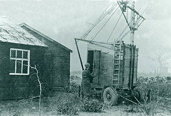
collide with molecules in the Earth's atmosphere and cause cascades of secondary particles and electromagnetic radiation that we call extensive air showers.] Initial observations at the University were blighted by interference from the trams running along the nearby street and so he got permission to set up his equipment at the Botany Department's proving grounds at Jodrell Bank some 20 miles south in the Cheshire countryside, Figure 10. He and his colleagues soon realized that the radar echoes that they were investigating were coming from meteors rather than from cosmic ray showers and much work was done, allowing the direction, velocity and orbits of the meteors to be determined. A second radio astronomy research group was set up at the Cavendish Laboratory at Cambridge under Martin Ryle whilst other groups began their researches in Holland, Australia and the USA.
Let us look in detail at some of the developments made by these research groups in the years immediately following the war.
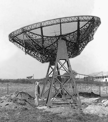
Jodrell Bank, UKThe most significant development made in the early years at Jodrell Bank was the building of a 218ft fixed parabola made up of a wire mesh surface laid on a grid of wires suspended from scaffold poles and guyed down to the ground to take up the correct parabolic profile. The guying system is in contrast to a mesh which when hung freely adopts a different profile termed a catenary. The feed system was mounted on top of a 126 ft mast, Figure 11. As the Earth rotates a thin strip of the sky is brought directly overhead through the beam of the antenna. Operating at a wavelength of 1.87m the beam of this telescope was about 2 degrees across, (make sure you can derive this value, 1m is 3.28ft, remember the actual value will be somewhat larger than that given by the "ideal" formula with the constant 1.22) this then being the resolution of radio maps produced by the telescope. By adjusting the guys that supported the mast it was possible to "steer" the telescope so that, in time a broad strip of the sky that comes overhead at the 53 degrees latitude of the observatory could be observed. By 1955 many discrete sources had been discovered, including the radio remnant of Tycho's 1572 supernova in Cassiopeia, and a survey giving the positions of 23 sources had been published. In contrast to these intense radio sources, Hanbury Brown and Cyril Hazard were also able to detect radio noise from the Andromeda Galaxy and, due to its 5 degree angular size compared to the 2 degree beam of the antenna, were able to make the first ever map of the radio brightness distribution of an individual radio source (remember the Sun and Moon are only 0.5 degrees across). Andromeda is a "normal" galaxy, like our own Milky Way galaxy, and the radio emission was shown to be very similar. The success of the 218ft paraboloid spurred Bernard Lovell in his quest for the building of a large fully steerable radio telescope that could be used to observe all parts of the sky. Cambridge, UK
Even a very large radio telescope such as that at Jodrell Bank had such a
broad beam that it is impossible to accurately locate a radio source in the
sky - important if one is to try to identify it on a photographic plate.
This is a fundamental problem in radio astronomy due to the fact that radio
waves are typically 100,000 times longer than light waves (wavelengths in
the visible part of the electromagnetic spectrum are around 500 nanometres i.e. 5x10⁻⁹m). The laws of optics (which apply to radio
waves just as well as light waves) require that in order to get the same resolution as an optical telescope a radio telescope would therefore have to be 100,000 times greater in diameter. If one considers even a small optical telescope one might have at home of 5cm in diameter, the comparable radio telescope would have to be ~5 km across! At this time the largest was the Jodrell Bank
218-ft (66 metres) antenna. An answer to this problem was provided by Martin Ryle at the Cavendish Laboratory of Cambridge University. With his colleagues, including Francis Graham-Smith
(later to become Astronomer Royal and Director of Jodrell Bank Observatory -
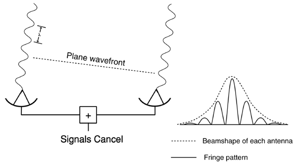
now an emeritus professor at Jodrell), he developed the technique of combining the signals of two or more antennas together to form what is called an "interferometer". This is simply a radio wavelength analogue of "Michelson's Interferometer" or, inversely, the "Young's Slits experiment" in optics. The signals received by the two telescopes are brought together and combined. If the signals are in phase, i.e. the peaks and troughs in the wave arrive at the same time, they will combine (or interfere) constructively and the resultant signal will be greater. If, on the other hand, the signals are out of phase by exactly 180 degrees (half a wavelength) they will interfere destructively and no signal will result if the two antennas are of equal collecting area.
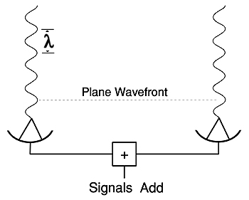
To illustrate this technique, suppose that two identical antennas sited on an east-west line are pointing due south as a radio source passes across the meridian (the meridian is the imaginary line drawn on the
sky between points on the northern and southern horizon and passing through the point directly overhead, the zenith). If the cable lengths from the two antennas to the point where their signals are combined are equal, then the signals will arrive there having travelled precisely the same distance from the source. They will thus arrive in phase and interfere constructively giving a maximum on a chart recorder plotting the received signal strength, see Figure 12. However, as the source moves past the meridian, the path lengths will begin to differ and the two signals will go out of phase until they interfere destructively and no signal is received (Fig. 13 left).
The path difference continues to change and the signals will come back into phase until a second maximum occurs and so on. The chart recorder will thus produce a trace which moves up and down called a fringe pattern. (This is analogous to the fringe pattern produced in the Young's slits experiment.) There is a second effect: as the source moves across in front of the two antennas it will first move into and then out of their beams. This gives a change in the amplitude (overall height) of the fringe pattern making it possible to tell which is the central maximum (Fig. 13 right). This is how we can use an interferometer to give a more precise position than would be possible with either of the individual antennae themselves. In the case of the single antenna we might be able to measure the position of the source to perhaps one tenth of its beamwidth. But with the interferometer we could measure it to one tenth of the width of the central fringe, which is determined by the
separation of the two telescopes. So, if the telescopes were separated by 10 times their diameter then we could find the source position to 10 times greater precision. The use of interferometers will be discussed in much greater detail later in the course but this should allow you to appreciate one reason why they are so useful.
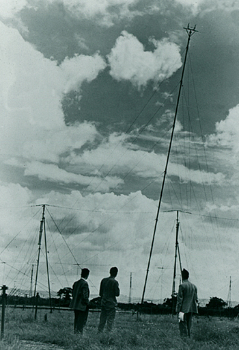
In a highly significant observation, Francis Graham-Smith used an interferometer made up of two WWII ex-Nazi Wurzburg 7.5m parabolic dishes to obtain the first really accurate positions of a radio source, Figure 14. In 1951 he measured the position of the radio source called Cygnus A that had been first discovered by Hey's group in 1946. He was able to find the Right Ascension (the celestial equivalent of longitude on the Earth's surface) of the source to 1 arc second and the Declination (equivalent to latitude) to 1 arc minute. This enabled Baade and Minkowski to identify it on photographic plates taken with the 200" Mount Palomar optical telescope. Barely visible because of its great distance, it appeared to be an unusual pair of interacting galaxies, but it is now known that its split appearance is due to a thick band of obscuring dust lying across a single galaxy. Its distance was shown to be over 100 million light years and it soon became apparent that radio telescopes would provide a tool for investigating parts of the universe that were so distant that they were beyond the reach of optical telescopes for several decades. This was the first identification of what is called a "Radio Galaxy" - one in which the emission of radio waves is vastly greater than normal galaxies such as our own and M31, the Andromeda galaxy. Their properties and the source of their radio emission will be the subject of a later course module. In contrast, his accurate position of the radio source Cassiopeia A (or Cas A) corresponded to a network of filaments within our own galaxy and is a supernova remnant - the remains of the massive explosion at the end of the life of a giant star. These observations showed the potential of this type of radio telescope. Their development at Cambridge for use in producing radio source surveys and later the building of large interferometric arrays will be covered in great detail later in the course. Australia
After the war the Australian group who had been developing radar systems began to use their technology to study both the ionosphere and the Sun. J.S. Pawsey discovered that the Sun produced two distinct type of radio emission associated with the "quiet" and "active" Sun. He was able to measure the effective temperature of the quiet sun and found it to be a million degrees Kelvin - vastly higher than the Sun's surface temperature of 6000 K. This corresponds to the temperature of the Sun's corona for whose
very high value there is, as yet, no definitive explanation although it seems related to
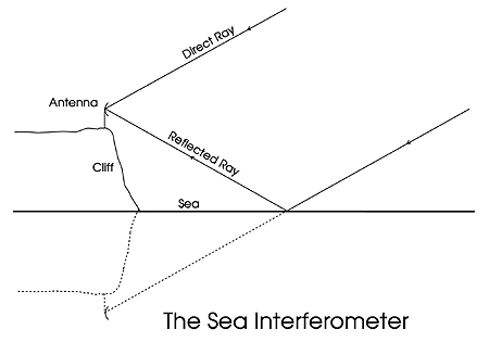
the energy which may be derived from the tangled magnetic fields which are threaded through the tenuous ionised plasma making up this part of the solar atmosphere. The Sun's emission increased several times when sunspots were present on the surface and, using a clever interferometric technique, he was able to show that the emission was associated with the sunspots. He built an analogue of the "Lloyd's Mirror" optical system in which he used one antenna mounted on a cliff facing east, Figure 15. As the Sun rose its radio signals would reach the antenna both directly but also by reflection off the sea's surface. This gives the effect of having two antennas one above the other and separated by twice the height of the antenna above the sea.
Bolton and Stanley used the same instrument to detect many of the first radio sources (then called radio stars!) and found the position of a strong radio source in the constellation of Taurus (Taurus A). This corresponded in position to the Crab Nebula - the remnant of the supernova observed in 1054 by the Chinese. This remnant, discovered optically in the 1700's is the first object, M1, in Charles Messier's famous catalogue. They later discovered the positions of several other radio sources, notably two radio galaxies Centaurus A and Virgo A. This latter corresponds to the giant elliptical galaxy, M87, at the heart of the Virgo cluster.
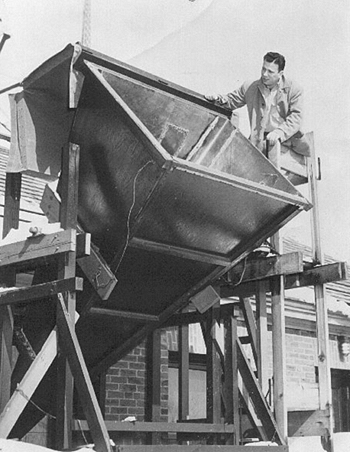
USAPerhaps surprisingly given the pioneering work of Jansky and Reber, radio astronomy as a research field did not really take off in America until the late 1950's when the National Radio Astronomy Observatory (NRAO) was established at Green Bank in West Virginia but, nevertheless, there were some significant developments. In September 1951 Ewen and Purcell used a small horn shaped antenna at Harvard University to detect the 21 cm line, Figure 16. The horn is now on display at NRAO and Ewen and Purcell shared the first Nobel Prize awarded in the field for their discovery. As we will see, this work, initially continued by the Dutch and Australians, eventually allowed the structure of our galaxy to be determined, enables the mass of other galaxies to be deduced and allow us to study the dynamics of galaxy clusters. At the famous Radiation Laboratory of the Massachusetts Institute of Technology (MIT), R. H. Dicke devised a method of continuous calibration of the radio receivers used in radio astronomy. In those days, the receiver noise generated by random electron currents within the receiver was far greater that the incredibly weak signals that came from all but the most intense radio sources. The meant that the passage of a weak source through the beam of a telescope could be masked simply because of changes in the receiver noise. Dicke invented a simple device, called the Dicke switch, to eliminate this receiver stability problem. In effect, the system continuously calibrates the receiver against a constant noise source derived from a resistor. This greatly improves the sensitivity of the receiver system allowing far weaker radio sources to be detected reliably. Techniques based on this simple switching idea are used in virtually all radio astronomy systems today. Americans pioneered the study of the Solar System. At the Naval Research Laboratory, C.H. Meyer measured the thermal emission of Venus at a wavelength of 3 cm. It corresponded to a temperature of 600K and thus implied an extremely hot surface. This was the first evidence of the "greenhouse effect" caused by the thick carbon dioxide atmosphere - to be confirmed far later by the Russian probes that landed on the surface. Further observations provided surface temperatures for Venus, Mars and Jupiter.
At the Carnegie Institute in Washington, Bernie Burke and K.L Franklin made the chance discovery of radio noise bursts coming from Jupiter as the inner satellites pass through the intense Jovian magnetosphere (the region dominated by the Jovian magnetic field). They had chosen to observe Jupiter at a frequency of 20 MHz, which it later transpired was at the centre of one of the narrow bands of Jovian radio emission.
NetherlandsFollowing on Van de Hulst's prediction of the 21cm Hydrogen Line at Leiden, it was not surprising that the earliest observations, using salvaged wartime radar antennas, were aimed at its detection. Success was achieved in 1951, close on the heels of its first detection at Harvard. The Dutch group pioneered the construction of fully steerable parabolic antennas and in 1956 completed a 25m antenna at Dwingeloo in northern Holland, Figure 17. The success of this instrument led to the construction of an impressive array of antennas to build the Westerbork Synthesis Array to be described later.
Recently, in its last years of operation, the Dwingeloo antenna detected the
presence of a previously unknown galaxy in our local group of galaxies by its
hydrogen line emission. Beyond the far side of our galaxy it had remained hidden
from optical telescopes by the obscuring dust along the plane of the milky way.
This highlights one great advantage of radio observations over optical - the
radio waves being so much longer than light waves can penetrate the dust and
thus allow radio astronomers to penetrate into regions unaccessible to optical
telescopes.
A summary of key points in this module
In the next module we will review some of the observations of thermal sources including "normal" stars like the Sun and a few more exotic objects.
|