Introduction to interferometric data
This guide provides a basic example for calibrating e-MERLIN C-Band (5 GHz) continuum data in CASA. It has been tested in CASA 6.5. It is designed to run using an averaged data set all_avg.ms (1.7 G), in which case you will need at least 5.5 G disk space to complete this tutorial. This tutorial is based upon the DARA 3C277.1 tutorial but is using new 2019 observations of the sources and some updates for ERIS 2022. If you find bugs in the code please contact Jack Radcliffe (jack.radcliffe@up.ac.za).
If you have a very slow laptop, you are advised to skip some of the plotms steps (see the plots linked to this page instead) and especially, do not use the plotms options to write out a png. This is not used in this web page, but if you run the script as provided, you are advised to comment out the calls to plotmsor at least the part which writes a png, see tutors for guidance.
Table of Contents
Important: The numbers in brackets respond to the steps in the accompanying python scripts.
1. Guidance for calibrating 3C277.1 in CASA
1A. The data and supporting material
For this workshop, we need the following files. These should have been included in the ERIS22_calibration_tutorial.tar.gz you should have downloaded. Un-tar this bundle (e.g., tar -xvf ERIS22_calibration_tutorial.tar.gz) and please double check that you have the following in your current directory:
all_avg.ms- the data (after conversion to a measurement set).3C286_C.clean.model.tt0- used for fluxscaling of the data set.all_avg_all.flags.txt- all flags3C277.1_cal_outline2022.py- the script that we shall input values into to calibrate these data.3C277.1_cal_all2022.py.tar.gz- cheat script for calibating these data.
.tar.gz or .tar) so you need to use tar -xzvf <filename> to untar these.
1B. How to use this guide
This user guide presents inputs for CASA tasks e.g., gaincal to be entered interactively at a terminal prompt for the calibration of the averaged data and initial target imaging. This is useful to examine your options and see how to check for syntax errors. You can run the task directly by typing gaincal at the prompt; if you want to change parameters and run again, if the task has written a calibration table, delete it (make sure you get the right one) before re-running. If you have done the CASA test tutorial then you can review the plotms command by typing:
# In CASA
!more plotms.last
This will output something like:
vis                  = 'all_avg.ms'
gridrows             = 1
gridcols             = 1
rowindex             = 0
colindex             = 0
plotindex            = 0
xaxis                = 'uvdist'
yaxis                = 'amp'
yaxislocation        = ''
selectdata           = True
averagedata          = True
transform            = True
extendflag           = False
iteraxis             = ''
customsymbol         = []
coloraxis            = 'spw'
customflaggedsymbol  = False
xconnector           = ''
plotrange            = []
title                = ''
titlefont            = 0
xlabel               = ''
xaxisfont            = 0
.....
As you can see in the script, the second format (without the #) is the form to use in the script, with a comma after every parameter value. When you are happy with the values which you have set for each parameter, enter them in the script 3C277.1_cal_outline2022.py (or whatever you have called it). You can leave out parameters for which you have not set values; the defaults will work for these (see e.g., help(gaincal) for what these are), but feel free to experiment if time allows.
The script already contains most plotting inputs in order to save time. Make and inspect the plots; change the inputs if you want, zoom in etc. There are links to copies of the plots (or parts of plots) but only click on them once you have tried yourself or if you are stuck.
The parameters which should be set explicitly or which need explanation are given below, with '**' if they need values. Steps that you need to take action on are in bullet points.
The data set that we are using today is a 2019 observation of 3C277.1, a bright radio AGN with two-sided jets. Within the data data set, named all_avg.ms it contains four fields that we are going to use to calibrate these data.:
| e-MERLIN name | Common name | Role |
|---|---|---|
| 1252+5634 | 3C277.1 | target |
| 1302+5748 | J1302+5748 | phase reference source |
| 0319+415 | 3C84 | bandpass, polarisation leakage cal. (usually 10-20 Jy at 5-6 GHz) |
| 1331+3030 | 3C286 | flux, polarisation angle cal. (flux density known accurately) |
These data have already been preprocessing from the original raw fits-idi files from the correlator which included the following steps.
- Conversion from fitsidi to a CASA compatible measurement set.
- Sorted and recalculated the $uvw$ (visibility coordinates), concatenate all data and adjust scan numbers to increment with each source change.
- Averaged every 8 channels and 4s.
2. Data inspection and flagging
2A. Check data: listobs and plotants (steps 1-3)
In this part, we shall see how we can get the information from our data set. One of the golden rules of data reduction is to know your data, as different arrays, configurations and frequencies require different calibration strategies.
- Firstly, check that you have
all_avg.msin a directory with enough space and start CASA. - Enter the parameter in step 1 of the script to specify the measurement set. The task
listobswill summarise the information given above and write it to a file namedall_avg.listobs.txt.
	listobs(vis='**',
			overwrite=True,
			listfile='all_avg.listobs.txt')
Important: To make it easier, the line numbers corresponding to the script 3C277.1_cal_outline2022.py are included in the excerpts from the script shown in this tutorial.
- When you have entered the parameter, we want to execute the step so that we run the task. In CASA you want to enter the following:
runsteps=[1]; execfile('3C277.1_cal_outline2022.py') - Check the CASA logger to ensure there are no errors (look for the word SEVERE) and check your current directory for a new file called
all_avg.listobs.txt. - Open this file using your favourite text editor (e.g., gedit, emacs, vim) and inspect it.
Selected entries from this listobs file, ordered by time, show the various scans during the observation,
  Date        Timerange (UTC)          Scan  FldId FieldName             nRows     SpwIds   Average Interval(s)    ScanIntent
	  01-Aug-2019/23:20:10.5 - 00:00:00.2     1      3 0319+4130                35820  [0,1,2,3]  [4, 4, 4, 4]
	  02-Aug-2019/00:00:04.0 - 00:00:07.0     2      2 1302+5748                   60  [0,1,2,3]  [3, 3, 3, 3]
	              00:04:54.5 - 00:06:01.0     3      1 1252+5634                  848  [0,1,2,3]  [4.14, 4.14, 4.14, 4.14]
	              00:06:04.0 - 00:07:59.5     4      2 1302+5748                 1484  [0,1,2,3]  [3.96, 3.96, 3.96, 3.96]
	  ...
	              09:30:03.0 - 10:00:00.2   183      3 0319+4130                12428  [0,1,2,3]  [4, 4, 4, 4]
	              10:00:03.0 - 10:30:00.2   184      0 1331+3030                16980  [0,1,2,3]  [4, 4, 4, 4]
	              10:30:03.0 - 10:32:00.3   185      2 1302+5748                  364  [0,1,2,3]  [4, 4, 4, 4]
	              10:32:03.0 - 10:36:01.0   186      1 1252+5634                 3220  [0,1,2,3]  [4.02, 4.02, 4.02, 4.02]
	              10:36:03.0 - 10:38:00.3   187      2 1302+5748                 1436  [0,1,2,3]  [4, 4, 4, 4]
	  ...
There are 4 fields:
Fields: 4
	  ID   Code Name                RA               Decl           Epoch        nRows
	  0    ACAL 1331+3030           13:31:08.287300 +30.30.32.95900 J2000        46256
	  1         1252+5634           12:52:26.285900 +56.34.19.48800 J2000       560340
	  2         1302+5748           13:02:52.465277 +57.48.37.60932 J2000       242296
	  3    CAL  0319+4130           03:19:48.160110 +41.30.42.10330 J2000        91856
Four spectral windows (each with 64 channels) with all four polarisation products:
Spectral Windows:  (4 unique spectral windows and 1 unique polarization setups)
	  SpwID  Name   #Chans   Frame   Ch0(MHz)  ChanWid(kHz)  TotBW(kHz) CtrFreq(MHz)  Corrs
	  0      none      64    GEO    4817.000      2000.000    128000.0   4880.0000   RR  RL  LR  LL
	  1      none      64    GEO    4945.000      2000.000    128000.0   5008.0000   RR  RL  LR  LL
	  2      none      64    GEO    5073.000      2000.000    128000.0   5136.0000   RR  RL  LR  LL
	  3      none      64    GEO    5201.000      2000.000    128000.0   5264.0000   RR  RL  LR  LL
And 6 antennas participating:
Antennas: 6:
	  ID   Name  Station   Diam.    Long.         Lat.                Offset from array center (m)                ITRF Geocentric coordinates (m)
	                                                                     East         North     Elevation               x               y               z
	  0    Mk2   Mk2       24.0 m   -002.18.14.1  +53.02.57.3      19618.7284    20856.7583     6908.7107  3822846.760000  -153802.280000  5086285.900000
	  1    Kn    Kn        25.0 m   -002.59.49.7  +52.36.17.2     -26823.2185   -28465.4973     7055.9694  3860084.921000  -202105.036000  5056568.917000
	  2    De    De        25.0 m   -002.08.40.0  +51.54.49.9      30300.7876  -105129.6730     7263.6278  3923442.718000  -146914.386000  5009755.292000
	  3    Pi    Pi        25.0 m   -002.26.43.3  +53.06.14.9      10141.4322    26944.5297     6845.6479  3817549.874000  -163031.121000  5089896.642000
	  4    Da    Da        25.0 m   -002.32.08.4  +52.58.17.2       4093.0417    12222.9915     6904.6753  3829087.869000  -169568.939000  5081082.350000
	  5    Cm    Cm        32.0 m   +000.02.13.7  +51.58.49.3     176453.7144   -97751.3908     7233.2945  3920356.264000     2541.973000  5014284.480000
In the next step, we are going to plot the positions of the antennae present in our observation. This is a handy way of getting a feel on the expected resolution and will assist when we try to determine a reference antenna.
- Take a look at step 2 and enter one parameter to plot the antenna positions (optionally, a second to write this to a png).
plotants(vis='**', figfile='**') - Execute step 2 by setting
runstepsand usingexecfilelike in step 1.
You should end up with a plot that looks similar to that below.
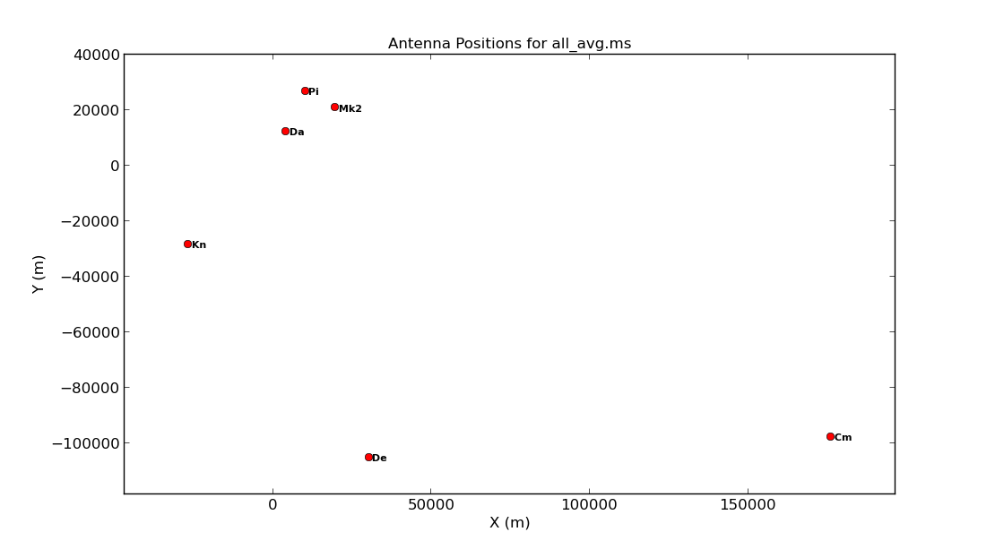
Consider what would make a good reference antenna. Although Cambridge has the largest diameter, it has no short baselines. We will use Mk2 for the reference antenna. Ideally we want all of the baselines to the reference antenna to look through similar atmospheric conditions so we typically choose the one with the shortest baselines, or we pick the most sensitive antenna.
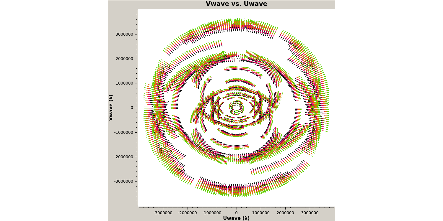
Next we want to plot the $uv$ coverage of the data for the phase-reference source so that we can see what Fourier scales our interferometer is sampling and whether we need to adopt our calibration strategy to adapt for snapshot imaging.
- Check out step 3 in the script. You need to enter several parameters but some have been done for you. Check out the annotated
listobsoutput above to try to identify these but remember to also use thehelpfunction,plotms(vis='**', xaxis='**', yaxis='**', coloraxis='spw', avgchannel='8', field='1302+5748', plotfile='', showgui=gui, overwrite=True) - Execute step 3 and check the new
plotmsgraphical user interface (GUI) that should have appeared on your screen.
Note that we averaged in channels a bit so that this doesn't destroy your computer. If this takes a long time, move on and look at the plot below. The $u$ and $v$ coordinates represent (wavelength/projected baseline) as the Earth rotates whilst the source is observed. Thus, as each spw is at a different wavelength, it samples a different part of the $uv$ plane, improving the aperture coverage of the source, allowing Multi-Frequency Synthesis (MFS) of continuum sources.
With our initial data inspection under way, we are now going to move onto finding and removing bad data that can adversely affect our calibration later down the line.
2B. Identify 'late on source' bad data (step 4)
The first check for bad data that we are going to look for is whether the antennae are on-source for the whole duration of the scan. This is important to check, especially for heterogeneous arrays, where the different slewing rates means that different antennae come onto source at different times. Often this is flagged automatically by the observatory but it is not always the case. The flagging of these data is called 'quacking' (don't ask me why!). Let's first plot the data to see if we need to quack the data!
- Check out step 4 and use
plotmsto plot the phase-reference source amplitudes as a function of time. To save time we want to select just a few central channels and average them. This needs to be enough to give good S/N but not so many that phase errors across the band cause decorrelation. Some hints on the proper parameter selection are given in the code block below.
	plotms(vis='**',
		   field='**', #phase reference source
		   spw='**', #plot just inner 1/2 channels for each spw (check listobs for the # channels)
		   avgchannel='**', #average these channels together
		   xaxis='**',yaxis='**', #plot amp versus time
		   antenna=antref+'&Pi',   #uses Mk2 as a reference antenna for comparison but other w/ short baselines are ok
		   correlation='**,**',  #just select the parallel polarisations as polarised intensity is fainter
		   coloraxis='corr', #colour by correlation
		   showgui=gui,
		   overwrite=True, plotfile='')
- Once you have inputted the parameters, execute step 4 and the plotms GUI should have opened
- Zoom in onto just a few scans and you should see a plot similar to that shown below.
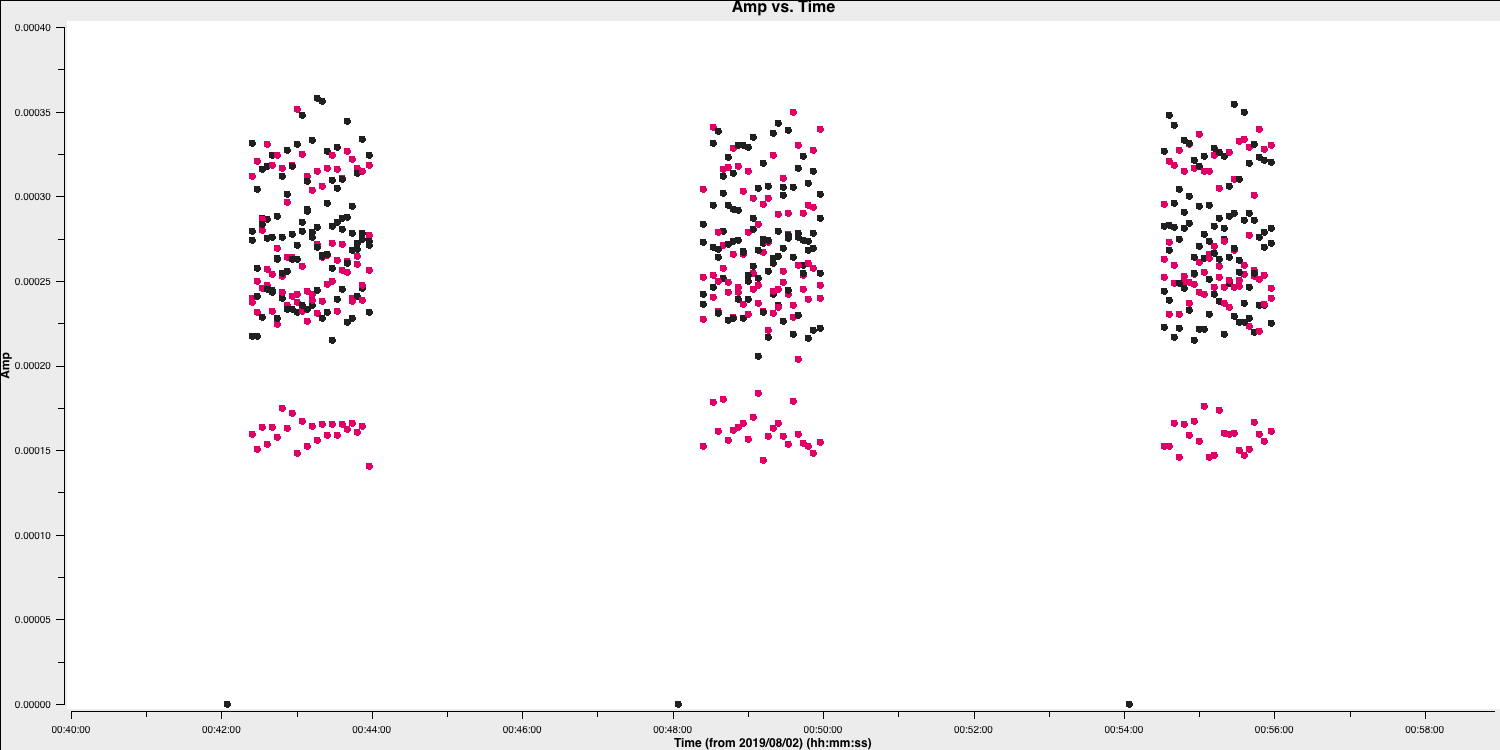
In this case, the pre-applied observatory flags which removed data when the antennae was off source was not perfect, resulting in the single integration at the start which needs to be flagged. This is roughly the same amount of time at the start of each scan is bad for all sources and antennas, so the phase reference is a good source to examine. (In a few cases there is extra bad data, ignore that for now).
- Estimate this time interval using the plot and we shall then enter that value in next part.
2C. Flag the bad data at the start of each scan (step 5)
One of the most important rules for good data reduction is good bookkeeping i.e., knowing exactly what has been done to these data, and how to return back to how the data looked in a previous step. Often you may find that you have entered an incorrect parameter and this has messed up your data, such as accidentally flagging all your data. CASA has some inbuilt methods to help with this bookkeeping. One of these is the task flagmanager which can be used to remember all the flags at a certain point in the calibration steps. This means that you can use this task to revert back to how the flags were before you changed them.
- Take a look at step 5, we are going to input parameters for both tasks before executing the step this time.
- The
flagmanagertask will be used to save the current state of the flags before we remove that bad data we identified at the start of the scans. Enter the parameters that will save the flags.flagmanager(vis='**', mode='**', versionname='pre_quack')
If the parameters are set correctly, then we will generate a backup named pre_quack in a all_avg.ms.flagversions file. After we execute step 5, you can check that it exists by running flagmanager again using mode='list' instead.
Next, we need to actually do the quacking or flagging of these channels. We use the CASA task flagdata to do this along with the special mode called quack.
- Fill in the
flagdataparameters, inserting the time that the antennas were off source that we found earlier.flagdata(vis='**', mode='**', quackinterval='**') #needs to be a integer - Execute step 5. The script will also re-run the
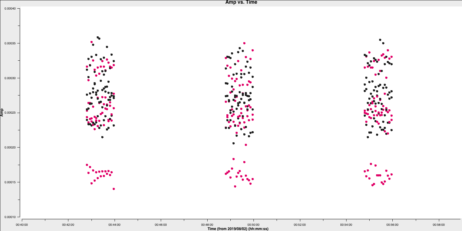
plotmscommand from step 4 to show that the data is removed (if your GUI is still open we could tick the reload option and replot it.)
This step should produce a plot similar to that below (when you zoom in) which shows the bad data removed.
2D. Flag the bad end channels (steps 6-7)
Due to limitations in the signal path, and the effect of dividing a continuous signal into spw and then taking Fourier transforms for correlation, the edges of each spw in the frequency domain are of lower sensitivity and are normally flagged. We often correct for this effect (called bandpass calibration), but the low S/N data on these edge channels can result in errant solutions and noise being injected into these data. This effect is instrumental and so is the same for all sources, polarizations and antennas. However, different spectral windows may be different. We need to look at a very bright source which has enough signal in each channel in order to see this effect. In this case we can use the source 0319+415.
To obtain the correct parameters for the flagging part, we want to identify the channels where the amplitudes versus frequencies are low so we want to plot these data.
- Look at step 6. For the
plotmscommand below. Add in the correct parameters to plot the frequency (or channel) for 0319+415.plotms(vis='**', field='**', xaxis='**',yaxis='**', #plot amplitude against channel antenna=antref+'&Kn', #select one baseline correlation='**,**', #just parallel hands (i.e. LL or RR) avgtime='**', #set to a very large number avgscan='**', #average all scans iteraxis='**', coloraxis='**', #view each spectral window in turn, and colour by correlation showgui=gui, overwrite=True, plotfile='')
The use of iteraxis allows us to scroll between the spectral windows (using the green arrow buttons in the GUI). Below is the plot for the first spectral window.
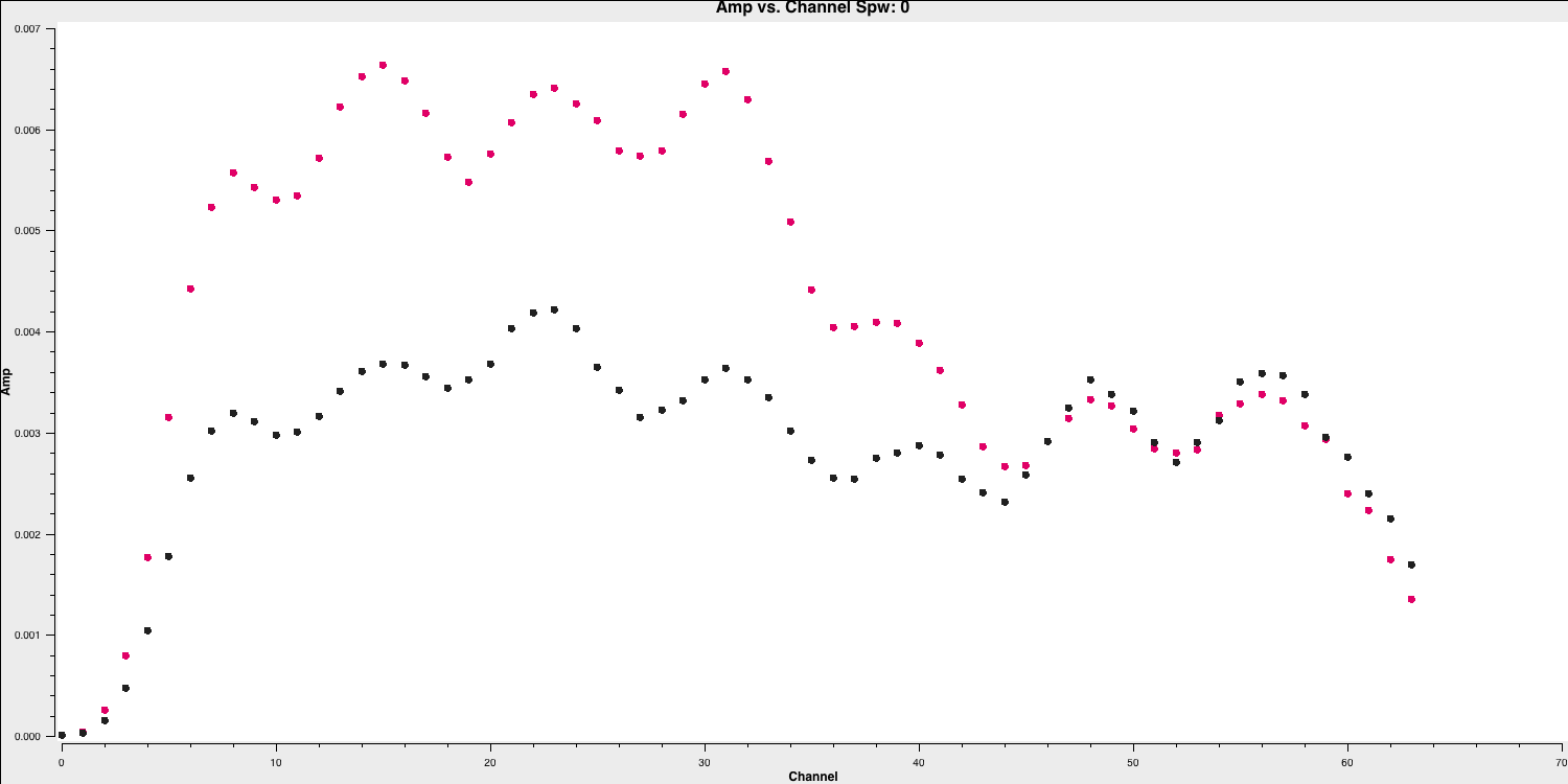
From looking at this plot we are going to flag the channels dropping off to zero at the edge. These are going to be approximately the first 5 channels (0-4) and the last three channels (61-63).
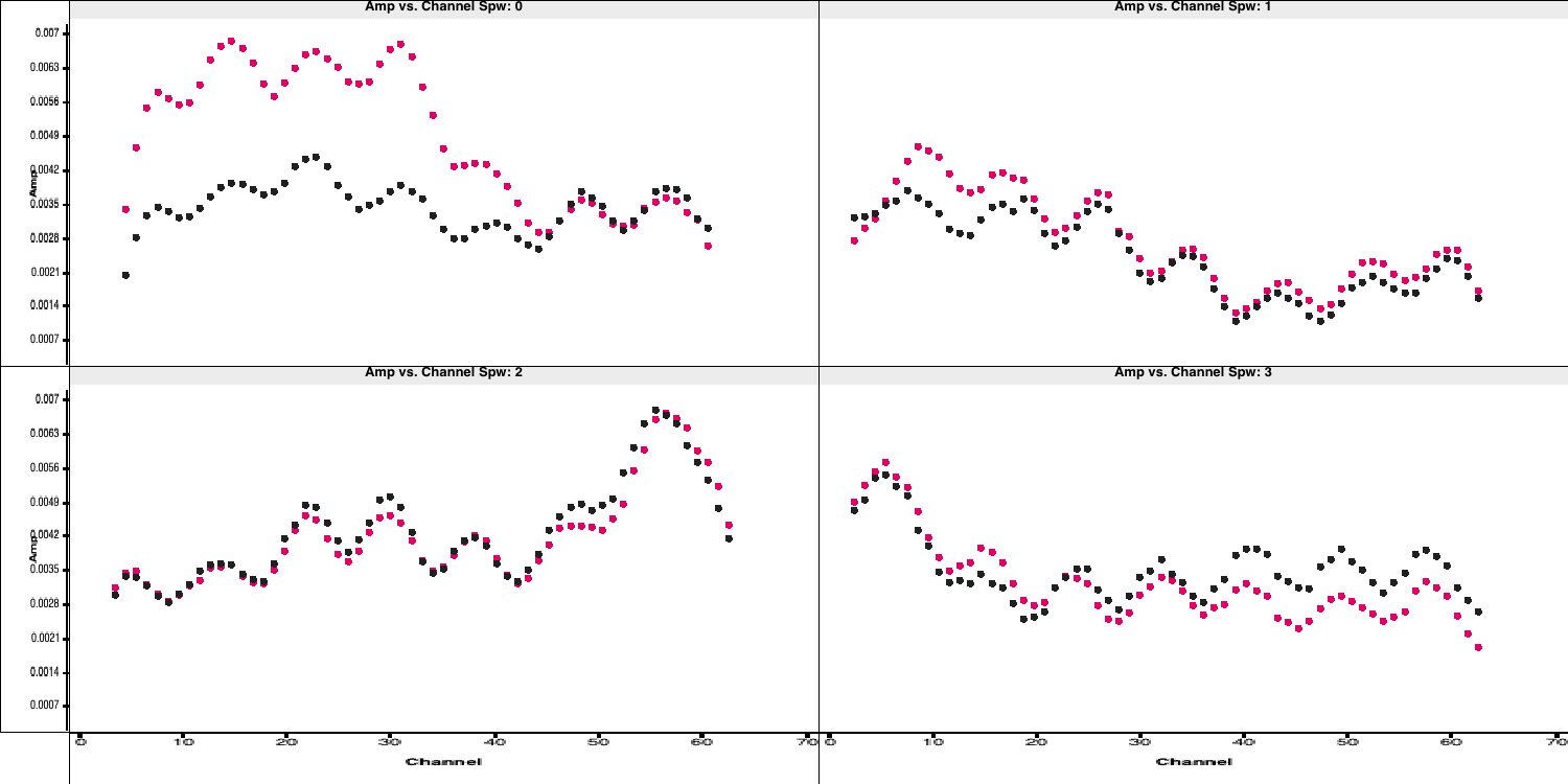
- Do the same for the other three spectral windows and note down which channels to flag (remember that we are using zero indexing so the first channel is 0).
With the channels for all spectral windows identified, we want to now actually flag them. However, remember that we should always back-up our flags should things go wrong.
- Look at step 7. Back up the flags and enter the appropriate parameters in
flagdata. Note the odd CASA notation for selecting spectral windows and channels. We have provided the "bad"/insensitive channels in spw 0 with the correct syntax, so use that as a guide for the other spectral windows. You can add multiple spectral windows in the same string using a comma e.g.,spw='0:0~3,1:0~4', will flag channels 0 to 3 in spectral window 0 and 0 to 4 in spectral window 1.flagmanager(vis='all_avg.ms', mode='save', versionname='pre_endchans') # End chans flagdata(vis='all_avg.ms', mode='manual', spw='0:0~4;61~63,***', #enter the ranges to be flagged for the other spw flagbackup=False)
- Execute step 7 and then re-plot in
plotms(the code should already do this replotting for you!). You should get a plot similar to that below
2E. Identify and flag remaining bad data (steps 8-10)
The final step in the flagging process is to closely inspect your data and look for other bad data. This can take many forms such as correlator issues (which causes low amplitudes on some baselines), antenna problems such as warm loads and Radio Frequency Interference (RFI) causing huge spikes in the data (plus many many more).
You usually have to go through all baselines, averaging channels and plotting amplitude against time and frequency. This can be very tedious so there has been considerable efforts to produce automatic flaggers (e.g., AOFlagger, rflag) which can do this automatically. However, you still want to judge whether these algorithms are working properly and not flagging decent data. Therefore having some experience doing it manually can give you experience on what exactly we consider as 'good' and 'bad' data.
To save time (and your sanity!), we are not going to do it all here. We are just going to look at one source, 0319+4130, and write down a few commands. This is done in the form of a list file, which has no commas and the only spaces must be a single space between each parameter for a given flagging command line. Some errors affect all the baselines to a given antenna; others (e.g., correlator problems) may only affect one baseline. Usually all spw will be affected so you can just inspect one but check afterwards that all are 'clean'. It can be hard to see what is good or bad for a faint target but if the phase-reference source is bad for longer than a single scan then usually the target will be bad for that intervening time.
Before we begin to flag, remember we should start by backing up the flags again!
- Take a look at step 8 and enter the correct parameters for
flagmanagerflagmanager(vis='**', mode='**', versionname='pre_timeflagging') - Take a look at the
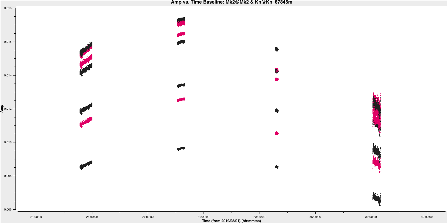
plotmscommands in the file. These will plot all the sources and save them to a file. The final command will put the amplitude versus time for 0319+4130, the source we want to flag now. - Use the
plotmswindow to inspect 0319+4130, paging (iterating) through the baselines. - Zoom in and identify the time ranges and antennae where we have bad data. Insert these into a text file and save that text file as
0319+4130_flags.txt. Some example commands are given below and a plot showing some bad data on 0319+4130 after zooming in is shown
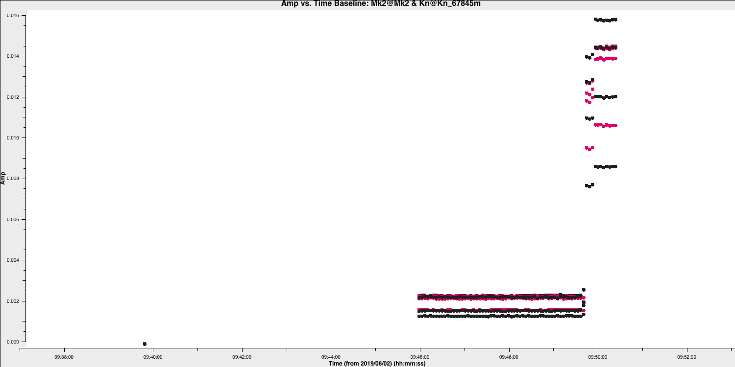
Here are some of the flagging commands in list format for the data shown below,
mode='manual' field='0319+4130' timerange='2019/08/02/09:30:40~2019/08/02/09:50:36'
mode='manual' field='0319+4130' timerange='2019/08/02/15:00:00~2019/08/02/15:05:40'
mode='manual' field='0319+4130' antenna='Cm' timerange='2019/08/02/15:18:18~2019/08/02/15:18:30'
By paging through all the baselines, you can figure out which bad data affect which antennas (i.e., the same bad data is on all baselines to that antenna. These commands are applied in flagdata using mode='list', inpfile='**' where inpfile is the name of your flagging file.
- Take a look at step 9, and enter the correct inputs into
flagdatafor you to apply the text file you have created. This step will re-plot the source to ensure that the data is now flaggedflagdata(vis='all_avg.ms', mode='**', inpfile='**') - Execute step 9 and inspect the plotting window. You should get a plot similar to that shown below.
- If you have time, expand your investigations to the other sources and enter flagging commands into your flagging file. You can then re-run step 9 to apply the new flags.
- If you are running out of time, take a look at
all_avg_all.flags.txtas theinpfilecommand and see how all the previous flagging commands can be applied at once. - Execute step 10 to apply these flags to ensure that your data is ready for the next tutorial: Calibration
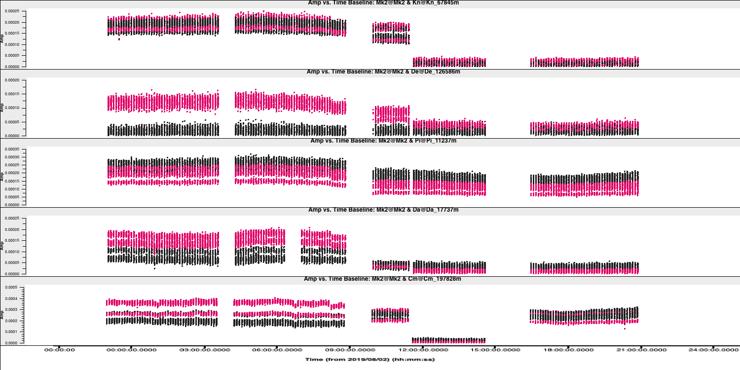
This step should also make some plots named <source_name>_flagged_avg_amp-time.png. Inspect these to check that all the bad data has been removed. A plot of amplitude versus time for the phase calibrator (1302+5748) is given below.
Congratulations, you have finished the first part of this tutorial. Next we shall move onto calibrating these data. Follow the link below to continue.