The science justification

These observations were proposed to image the neutral hydrogen via absorption against the inner radio jets of 3C293. 3C293, itself is a moderately large nearby FRI radio galaxy (see 1.4GHz VLA image with MERLIN inset) which has a complex inner radio jet with a lot of gas & dust in the middle (see here, here, or here). The size of this inner jet is ~5 arcsecond making it an ideal MERLIN target. At a distance of 180Mpc the 21cm line of H1 is redshifted to 1359MHz which is observable with MERLIN (current lower frequency limit for the MERLIN telescopes at L-band is 1330MHz, however these lower frequencies are often affected by radio interference, so beware).

Although neutral hydrogen is often observed in emission by many single dishes and lower resolution tied-arrays, such as the WSRT, VLA, GMRT & ATCA, its low brightness temperature, typically few hundred Kelvin, is below the sensitivity of the current generation of radio interferometers when observed on angular scales of <1arcsec. However, H1 can be observed at sub-arcsecond or mas resolutions via absorption against bright radio sources. These observations exploit this fact by observing the H1 within the host galaxy of the radio source 3C293 via absorption along lines of sight toward its bright radio continuum emission.

These data are published in R.J. Beswick, A. Pedlar & A.J. Holloway 2002, MNRAS, 329, 620.

The observations

This observation was made using 6 MERLIN telescopes (Defford, Cambridge, Knockin, Darnhall, Mk2 and Tabley) on the 8th April 1998. Both left and right hands of circular polarization were measured each with 8-MHz bandwidth. The data were then correlated into 64 channels in frequency, each with a bandwidth of 125 kHz, resulting in a velocity resolution of 26.3 kms^-1. Frequency channel 32 was centred upon the optical-heliocentric velocity for 3C293 (13500 kms^-1).

The observations were made over 18 h, regularly interspersed with observations of OQ208 which was used for phase calibration. OQ208 was also strong enough (0.7 Jy) to be used for bandpass calibration. An observation of 3C286 at either end of the run of observations was used to calibrate the absolute flux density scale of the observations. This was achieved by assuming that 3C286 has a flux density of 15.05 Jy at 1359 MHz.

The Data

The primary purpose of this tutorial is to image these spectral line data and manipulate the resulting data cube. This tutorial has been designed so you need not start at the begining, as there are fits files that you can download along the way if wish to skip over some steps.

The calibration of these data has basically followed the same techniques as were discussed in the Wide field imageing and in basic calibration sections. These data do have significant radio continuum and can be have been phase referenced, the data averaged in frequency and self-calibrated on the strong radio continuum target. The only difference between these data and normal continuum data is that we have then applied this calibration to the unaveraged (in frequency) data set and we have also applied a bandpass correction based on our point source calibrator OQ208 (which was also observed as a phase reference source and thus has very good signal to noise).

Within aips a list of all spectral line related tasks/verbs/adverbs can be obtained by typing 'About spectral'. This can be a useful memory aid to find the task that does what you want to do!

Stage 0: Loading these data

The relivant fits file should all be on the system already, if not they can be downloaded via the links listed along the way. Then as you did in the previous tutorials set a soft link to the data area and use fitld to load the fits file. Note that all of these fits files have lower case letters in their names. To load these into AIPS you can either mv the files to a name that is all capitals or leave off the end apostrophe in the infile statement (e.g. DATAIN 'WORK:this_fits_file.fits).

Stage 1: Spliting the data

Split the multi-source UV file into a single source file. Applying the calibration.

Basic aips inputs are as follows:
Task 'split' $ Split the multi-source UV file into a single source file. Applying the calibration.
getn i $ i=catalog number of the mulltb file
sources '3C293' '' $specify the source you wish to split out - the target
docalib 1;gainuse 0;doband 1;bpver 0
bchan 1
echan 63
nchav 1
ichansel 1 63 1
go split
**(This stage can be skipped by loading in the split.fits file rather than the multtb file)

Define the velocity-frequency conversion.

These observations have multiple spectral line channels each of which is recorded at a different frequency. At this stage we are just confirming definition of the velocity information in the header so that on our latter mapped images we can convert from frequency to velocity. Use the verb 'altdef' to define the reference velocity. For these observations the rest frequency is that of the H1 line and the centre chanel has been shifted to a frequency that is equivalent to 13500km/s.

AIPS inputs
getn i+1 $ (split file)
AXTYPE 'OPT HEL ' ;AXVAL 13500000 0
AXREF 32
RESTFREQ 1.420E+09 4050000
ALTDEF

Note this the centre channel in the whole band is channel 32. The experiment was tuned so that the centre channel was at 13500 km/s.

Following the imageing of these data we can now type altsw in aips to convert between velocity and frequency for our 'third' axis of any data cube.

Note that these observations have already been corrected for the motion of the earth over the obervation period.

Imaging & continuum subtraction the spectral line data

This is covered in more detail in Synthesis image in Radio astronomy II, chapter 12.

WHY?
The reasons for subtracting the continuum are many. Firstly, and most simply it is far easier to see a spectral line (emission or absorption) in a specific spectral channel when emission common to all channels is removed. Secondly, removing the continuum minimizes, and sometimes eliminates, the effort involved in deconvolving the line signal, since it removes the need to deconvolve the same continuum emission from every channel. This is a good thing because deconvolution is inherently non-linear, and can give different results for different channels simply because of the u,v coverage and noise can be different. Similarly a better continuum image will result in averaging together the line-free channels before decovolution.

HOW?
1) Subtraction in the Map plane.

Firstly make a dirty spectral line cube from the split file. This can be done using imagr. Do not clean this data at this stage (ie. set niter =0). Since this is a spectral line data set we do not wish to average the channels.

Some specific imagr settings:
outnam '3c293.dirty'
bchan 1;echan 63;nchav 1;doband -1;imagrprm(10) 1
niter 0;robust 7;docalib -1
imsize 512;cellsize 0.04;minpatch 255

This will create a dirty image cube and beam cube, check the map header of these two files they should have 63 frequency channels in the third axis. Note that the begining and end channels are bad. (3C293_MERLIN.dirty_cube.MA.fits & 3C293_MERLIN.dirty_beam.MA.fits )

Inspecting the dirty cube
At this point it is a good idea to inspect the image cube. Spectral line cubes can be displayed using various task within aips. Brief explanations of some which may be useful can be found here. At this stage we need to know which channels contain line and which are line-free so we can subtract the continuum (ispec is a useful task for this).

The source 3C293 has fairly strong radio continuum, so it should be 'relatively' easy to see the absorption even in the dirty unsubtracted cube. Taking an ISPEC against the inner jet/lobes of the dirty cube you will see the absorption is strong (dirty-specEAST.pdf & dirty-specWEST.pdf ). Notice in the spectra there appears to be two sets of absorption lines, on in the centre an one blueshifted. Also notice the shape of this blueshifted line does not change significantly across the source. This second off-centre line is actually RFI, confirmed since it is visible on the phase calibrator too! (see here ).

Once you have selected you line (& RFI free channels) use the aips task IMLIN to subtract the continuum. Note that the cube must be transposed before imlin will work, using trans, so that its axis order is freq,ra,dec [312]

Some specific imlin settings:
infile ''
box 5 20 40 48
nboxes 2
order 1 $ ie. use a constant slope rather than try to fit a polynomial
dooutput 1

When this is completed you will have a dirty by continuum subtracted cube. Note that it will be axis ordered freq, ra, dec [312] - So you will need to use trans to re-order the cubes axis to make it clearer what you are looking at (this is needed for the next step anyway). Inspect this cube to check that imlin has worked correctly.(see spectra ).

Cleaning the cube
If you tvmovie through the transposed (ra,dec,freq [123]) you will notice that the line is quite strong and still needs to be cleaned.

Clean the cube for example using the task apcln. Apcln is an old aips task and not recomended but this task will clean images.

Some specific apcln settings (running with a loop):
Set all of your outnam,outclas, outseq to a specific unique name - or you will fill you disk up.
getn i $continuum subtracted cube"
get2n j $dirty beam
outnam '3c293.clean'
outclas 'rdfl-c'
outseq 1
niter 2000
blc 0
dotv -1
CHECK INPUTS
Then on the aips command line type:
for i=1 to 63;blc(3)=i;go apcln;wait apcln;end

this will run apcln 63 times, once for each channel, and write the cleaned files to one aips catalog number. If you have not specified the outseq number this will create 63 cubes each with one pannel of data and fill up your disk (s)! if so delete the files it has created (e.g. for i=x to y;getn i;zap;end --carefully!)

An example cleaned, continuum subtracted cube is 3C293_IMLIN_CLEAN_CUBE.MA.fits.

Now you should have a clean and continuum subtracted cube.

Because this is an absorption experiment you can also make a good image of the radio continuum. To do this use the '.CONT' file that imlin created and clean it. Remember that this time it is a single image not a cube, so there is no need to loop over every channel. But you will have to create an appropriate dirty beam, from you dirty beam cube, that is an average of the same channels. To do this imlin can be run with the same settings (tget imlin) on the dirty beam.

NOTE: for the more ambitious people, or those who wish to check what is going on, this continuum subtraction could also be done by using the task sqash to collapse the appropriate continuum channels down and then the task comb to subtract them from the cube by by hand. Imlin in essence does just this, but also allows you to fit a gradient to the continuum baseline.

2) Subtraction in the uv-plane
There are several aips task that allow you to subtract the continuum from your data in the u,v plane for example UVLSF,UVLIN. As discussed above in many way this is often a prefered method, compared to subtraction in the image plane.

To demonstrate this we can run UVLSF on the split file. Firstly we need to select the ichansel to specify the line-free channels to represent the continuum.

Some specific uvlsf settings:
bchan 1;echan 63 $ Include all channels
ichansel 5 20 1 40 48 1 $ fit to these windows where there is just continuum.
order 1
dooutput 1 $ will create a averaged continuum u,v data set

UVLSF will create two files (if dooutput=1). The '3C293_MERLIN_UVLSF.UV.fits' file is a u,v continuum subtracted multi-channel data set, whereas 3C293_MERLIN_BASFIT.UV.fitsis the fit to the continuum subtracted (ie a single channel uv file).

Both of these files can be cleaned using, for example imagr.

Some specific imagr settings (cleaning the multi-channel data):
bchan 1
echan 63 $(or what ever is the last channel in you data)
nchav 1
Robust 7 $ or what ever weighting you desire.
dotv -1 $ you got to do the tv thing 63 times otherwise!
niter 2000 $ Less would be reasonable since you have only line signal to clean.

Also clean yourself a continuum image, you probably want to do this interactively. Note use the same cell and image size for both the continuum image and line cube. - To do this run imagr on the basfit uv-file that UVLSF will create.

This is the continuum map as a contoured image or 3C293_CONT_BASFIT.MA.fits.

Manipulating & Displaying the Spectral line cube

A continuum sub-image 3C293-SUBIM.ICLN.MA.fits.

Using the same blcs and trcs do the same with the spectral line cube. However in the case of the spectral line cube you will need to add a third number (replace the 0 above) which represents the number of channels to be included. Use ISPEC (ltype 6) to choose how many channels to include, remember to exclude any end channels where the band drops away and also at this stage exclude the RFI signal toward the righthand side of the band. Example, if you have a 512x512x63 cube settings might be blc 150,150, 8;trc 350, 350, 50.

A continuum subtracted, cleaned sub-cube 3C293-SUBIM.ICLN.RDFL-C.MA.fits.

Converting your frequency axis to velocity
The frequency axis of the cube can be converted to velocity. Earlier we defined this in the header information using axdef. Now to switch between frequency and velocity just getn the cube you wish to convert and type ALTSW. Note that frequency and velocity axis obviously run in the opposite direction, so whereas frequency grew with channel number the velocity will reduce. If you wish to flip this axis around this can be done in trans by applying a transcod '12-3' for example.

Viewing the cube
Use TVMOVIE/TVCUB/TVALL to view the continuum subtracted cube. Look to see where the absorption signal is. How does it alter as you travel through the cube.

Making spectra from the cube
Firstly to make indiviudal spectra of a selected area the aips task ispec is very useful. On any cube select the area/pixels over which you wish average to make a spectra. Since there is no no continuum in you lie free cube you may wish to tvlod your matched size continuum image and use this to select the regions of interest with tvwin. Then either with DOCRT=1;DOTV =1 or -1(if you wish to view the spectra on the TEK screen) type go ispec. Ispec will produce a list of numbers to the command line which can be written to a text file if you wish, and will produce a plot of the spectra.

Try using the task plcub. This will create a grid of spectra over a specified area. To run this task you will need use a transposed version of the continuum subtracted cube. PLCUB only plots spectra at a single pixel rather than averaging over an area, so you will need to set YINC=i & ZINC=j so that it plots the spectra for every ith and jth pixel in RA & dec. Remember to reset yinc & zinc after using them.

Contouring the cube Try using KNTR to contour the continuum subtracted cube. You can use kntr to simultanously contour a selected range of channels.

Moment analysis
One of the most common methods used to establishing the gas distribution, velocity field and line width of a spectral line signal is to calculate the moment of the line profile. Here is an example of a moment 1 map of H1 absorption against NGC3079 obserevd with MERLIN.

For much more information see ASP180, page 262-268. The moments of the line profile are calulated as follows:

Moment 0 (line intensity)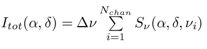

Moment 1 (velocity)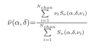

Moment 2 (velocity dispersion)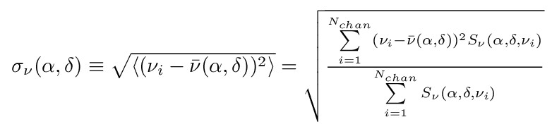
higher moments such as kurtosis of the line can also be calculated.

Note that the higher moments depend upon the lower orders, so higher orders will become progressively more noisy. Moments have several other issues you should be aware of when interpreting them. For example if there are multiple components, or two lines (eg. observations of OH) moments are can be very difficult to interprete or misleading. If there is both absorption and emission present the two can be summed together and so on. All these factors do not mean that moments can not be very useful and meaningful but does mean they should not be used blindly.

Within aips there are two task which can perform this MOMNT and XMOM. Both of these will work on a transposed continuum subtracted cube. Try running them on your sub-cube. The key things to remember are to include the channels with line signal, with minimal other channels (use blc,trc) (ie do not include begining and end channels). Set the icut value to be just above the noise level in each channel so that only line signal is included (try various icut values to see which turns out best). Plus since this is an absorption experiment set Flux =-100, so that it includes things below zero.

To get a better result we can use some a prior knowledge. Since this is an absorption experiment we would not expect to any absorption were there is no continuum. So we can use the radio continuum image, blanked at a certain value as a template to blank the cube in all areas where there is no continuum. This can be done by passing the continuum image through blank with opcode 'selc' and the appropriate cutoff levels set and then using this output as a template in blank (opcode 'in2c') to select the unblanked areas in the cube. 3C293-subim-BLanked_at_5mJy.MA.fits is a sub-cube with areas with less than 5mJy/bm of radio continuum blanked.

As you can probably appreciate, the complex nature of the absorption lines against the western half of this source means that moments do not do justice to this data but here is an example picture anyway.

Collapsing the cube in any direction
You can use sqash or xsum to collapse the cube along any axis. Firsly use trans to transpose and/or lgeom to rotate the cube so the axis you wish to average along is the third axis. In this sense you can make a 2-D averaged image of the cube along your choice of 'D' eg Ra vs velocity or what ever show off the data best. Here is a PV diagram made in this way from these data..

Recombining the radio continuum and the line
To create spectra for presentation you may wish to recombine the radio continuum and the spectral line data. In reality since this is an absorption experiment the strength of the line signal is dependent upon the strength of the background continuum. As such it often gives a more realistic presentation of the data if the radio continuum baseline level is included.

Try using the task 'comb' to add the radio continuum map to each plane of the cube. Set the blc 0 0 1;trc 0 0 i (where i is the number of channels in your cube), opcode 'sum';aparm 1 1 0;bparm 0. This will add your continuum fits file to each plane of you cube. Then view your cube and take spectra.

Making an optical depth cube

The intergrated of the absorbed H1 line is not just proportional to the amount of H1 along the line of sight but also the strength of the background continuum. As such to get a handle on the true amount of gas along the line of sight to the continuum you may wish to make an optical depth cube.

For a H1 absorption experiment this can be achieved as follows:-

To calculate the TAU for a source you need the continuum image(C) and the line+continuum (L+C)image:

1.TVWIN around SNR in question and SUBIM this bit off in both the C-image and the L+C-image. So you're left with a C-image square around the SNR and an L+C-image square around the source.

2.Work out correction for any missing zero-spacings (eg. using VLA map) and then add this value to both SUBIM'd images - ie add on the correction using MATHS to the L+C-SUBIM'd image around the source and the C-SUMIM'd image.

3.Check there are no longer any negatives in the L+C-SUBIM'd image - there shouldnt be.

4.Apply COMB using the corrected L+C-SUBIM'd image and the C-SUBIM'd image. I think you do this using TAU=-ln( (L+C-SUMIM'd image)/(C-SUMIM'd image) ) which requires aparm(1)=-1, aparm(2)=0, aparm(3)=1, aparm(4)=0

5. What you get out is a little TAU-map for that one SUBIM around that source. If you do an ISPEC on it you should be able to read off the value of TAU at the maximum point of absorption (when you run ISPEC these numbers are printed on the screen). This value is equivalent to TAU_peak.

Displaying & viewing a data cube: Some useful AIPS tasks