1.3 Dynamics of the Universe
1.3.1 The Friedman Equation
We have seen that in a homogeneous, isotropic universe the only change
allowed is an overall expansion or contraction, which is characterised by the
scale length R(t). The rate of change of
R (the "speed" of expansion of the universe) is written ![]() ,
but it is usually more convenient to work with the Hubble parameter H =
,
but it is usually more convenient to work with the Hubble parameter H = ![]() /R.
If we could calculate how R changes with time we would know the
whole past and future history of the Universe, at least on the largest scales.
On these scales the only force that acts is gravity, and the best available
theory of gravity, GR, gives the answer in the form of a surprisingly simple
equation, named in honour of the Russian cosmologist Alexandr Friedman
(1888-1925). The equation is:
/R.
If we could calculate how R changes with time we would know the
whole past and future history of the Universe, at least on the largest scales.
On these scales the only force that acts is gravity, and the best available
theory of gravity, GR, gives the answer in the form of a surprisingly simple
equation, named in honour of the Russian cosmologist Alexandr Friedman
(1888-1925). The equation is:

Here G is
To solve the Friedman equation and predict the
history of the Universe, we need to know:
- the
present energy density in the Universe,

- the
Hubble constant H0, which, with r(t0), allows us
to calculate the curvature constant k and R0 = R(t0)
which gives the scale on which geometry departs from
- the way the energy density changes as the Universe
expands, which depends on the type of "stuff" involved.
1.3.1.1 Derivation of the Friedman EquationRecall that the gravitational force between two objects with masses M and m, separated by a distance r, is F = -GMm/r2. This implies that the potential energy is V = -GMm/r. It is negative because we have to do work to pull the particles further apart (larger r). As ever, we assume that the universe is
perfectly homogeneous and isotropic. The idea is now to focus on the
behaviour of a small region, which of course will behave exactly like every
other region. First, we surround our chosen region with a
spherical surface of co-moving (dimensionless) radius Now consider two galaxies, one in the middle of
our sphere and one on the outer edge. From Hubble's law, we know that at a
given time they are moving apart at a speed v = Hr. Relative to
the central one, the second galaxy has a kinetic energy T = (1/2)mv2 where m is its mass, and a
potential energy V = -GMm/r
due to the gravitational field of the matter within the sphere (mass M).
From conservation of energy, T + V
is constant with time. We can write the mass in the
sphere M in terms of the average density of the universe, r,
times the volume of the sphere. This gives
Both kinetic and potential energy are proportional to the galaxy mass m,
and, on close inspection, to the square of the co-moving radius,
Dividing through by mr2/2, and
rearranging, we get
which is
(almost) the Friedman Equation. The one problem is that the constant C is unknown. From Newtonian gravity this is as far as
we can go. Einstein's theory supplies the constant: 2C = - kc2. Our Newtonian derivation assumed that the
universe was composed of ordinary matter, so that mass was conserved when our
sphere expanded. The real Universe did not behave like that at early times,
and recent discoveries suggest that it does not behave like that at the
moment. But it happens that the Friedman equation remains correct, provided
we interpret the density using Einstein's mass-energy equivalence, E =
mc2. That is, the effective mass density is defined by r= u/c2
where u is the density of energy in the Universe. |
1.3.2 What happens when the Universe expands
We
need to know how the density depends on the expansion of the Universe, which we
can specify by the scale length. That is, we consider density to be a function
of R: r(R). Since the volume of any bit of the Universe is
proportional to R3, this is equivalent to finding a formula
for density as a function of volume; such a formula is called an equation of state.
Exact equations of state tend to be very
complicated, but luckily almost all the time the equation of state of the
Universe is very close to a power law:
![]()
where the
power n depends on what type of matter is involved. For this type of
equation of state the pressure turns out to be
![]() .
.
Usually
we specify the equation of state by the value of w rather than n; notice that n = 3(w + 1).
1.3.2.1 Cold Matter
We
know that a particle with energy E has mass m = E/c2. This includes a component called the rest mass, m0, which is always present, plus extra mass
contributed by the kinetic energy of the particle. If the speed v is much less than the speed of light, the kinetic
energy is (1/2)m0v2, which is much less than m0c2, so the
energy is dominated by the rest mass. Since the speed of particles in a gas is
controlled by the temperature, we say that the matter is cold if v « c.
Even gas at 108 K is "cold" in this cosmological sense!
This is the case we assumed when deriving the
Friedman equation. The energy in a region bounded by fixed co-moving
co-ordinates (a co-moving volume) is the sum of the particle rest masses
inside, which is constant; and so the density is just proportional to the
inverse volume, i.e.
![]() .
.
With
n = 3, the pressure of cold matter is zero, or rather,
negligible compared to the rest mass energy density.
The simple way to find the proportionality
constant is to use the present-day values:

1.3.2.2 Radiation
Nearly
all the photons in the Universe belong to the Cosmic Microwave Background. They
were created soon after the Big Bang and, except for a negligible fraction
which run into stars, radio telescopes, etc, they are not destroyed. Although
individual photons move through the Universe, the number in a given co-moving
volume stays the same because equal numbers enter and leave (always assuming
homogeneity). Thus the number density of photons is proportional to R-3, just as for the number density ordinary
matter particles. But whereas the energy (= rest mass) of each matter particle
is constant with time, we have seen that all photons suffer a redshift, so the energy of each photon, hc/![]() , is proportional to 1/R. Thus the radiation energy density is proportional to
(density of photons) × (energy of each photon)
, is proportional to 1/R. Thus the radiation energy density is proportional to
(density of photons) × (energy of each photon)
![]() .
.
Radiation
has a pressure P = u/3. These equations are
exactly true for photons, but are also approximately correct for any particles
which are moving close to the speed of light, in which case special relativity
theory tells us that their energy is much greater than their rest mass energy.
For particles at temperature T, the typical energy per
particle is ![]() kBT, where kB is Boltzmann's constant.
Thus any kind of particle which is "relativistically
hot", i.e. kBT »
m0c2, counts as "radiation" as far as
the Friedman equation is concerned.
kBT, where kB is Boltzmann's constant.
Thus any kind of particle which is "relativistically
hot", i.e. kBT »
m0c2, counts as "radiation" as far as
the Friedman equation is concerned.
1.3.2.3 Dark Energy
Dark energy is a generic term for any kind of
stuff with negative pressure.
The prototype for dark energy was the cosmological
constant, usually represented by the Greek letter ![]() (Lambda),
corresponds to an effective density that is independent of R:
(Lambda),
corresponds to an effective density that is independent of R:
![]() .
.
This
implies w = -1, and hence, for positive ![]() , negative pressure: P = -u. In principle,
, negative pressure: P = -u. In principle, ![]() might be negative, which would not strictly count as
dark energy; but observations suggest a positive value, if any.
might be negative, which would not strictly count as
dark energy; but observations suggest a positive value, if any.
|
Figure 1.11: A cylinder full of 'Cosmological
constant' will exert a negative pressure on the plunger. |
![\begin{picture}(10,5.4)
% put(0,0)\{ framebox(10,5.4)\{ \}\}
\put(0,0){\includegraphics*[width=10cm]{lambdas.eps}}
\end{picture}](node4_files/image032.gif)
To see how peculiar this idea is, think of a
cylinder containing "![]() stuff" (Fig. 1.11).
If you pull out the plunger, increasing the volume filled by the
stuff" (Fig. 1.11).
If you pull out the plunger, increasing the volume filled by the ![]() stuff, you will have increased the energy in
the cylinder, as the density is unchanged and the volume is bigger. By
conservation of energy, you must have done some work; in other words, the
stuff, you will have increased the energy in
the cylinder, as the density is unchanged and the volume is bigger. By
conservation of energy, you must have done some work; in other words, the ![]() stuff must pull back on the plunger; it
corresponds to a sort of tension in space. This is the meaning of
negative pressure.
stuff must pull back on the plunger; it
corresponds to a sort of tension in space. This is the meaning of
negative pressure.
The original motivation for this strange idea was
that in 1917 Einstein found that, according to GR, a
universe containing only ordinary matter would inevitably expand or contract.
In an unusual failure of imagination, he refused to consider the possibility
that this might be happening, and instead proposed the cosmological constant to
keep the universe static.
For obvious reasons the cosmological constant fell
into disfavour when the expansion of the Universe was discovered; but since the
early 1990s, observations have increasingly seemed to be inconsistent with a
universe dominated by matter, and a cosmological constant seems to give the
best fit to the data, even though it is still as ad hoc as ever.
The idea of a cosmological constant irritates many
theorists, partly because a universal energy density which is strictly constant
in time and space has almost no effect on anything except the large-scale
expansion of the universe. This means that it is very difficult to imagine ways
of getting corroborating evidence for its existence. It also means that there
is no scope for elaborating the theory.
Therefore there is a lot of interest in the
possibility of a component of the Universe which behaves something like a
cosmological constant, but has more "interesting" properties. This
something has been named quintessence.
Quintessence is a material with equation of state
PQ = wrQ
with -1
< w < 0. This implies that the density depends on R according to:
![]() .
.
Our
earlier discussion shows that w = -1 corresponds to a
cosmological constant, and w = 0 corresponds to ordinary matter. Unlike the
cosmological constant, both the density and (in some versions) w may vary from place to place on small scales, just as
ordinary matter does. While all this makes life interesting again for
theorists, observations cannot yet distinguish quintessence from the
vanilla-flavour cosmological constant, and so we will mostly ignore this
possibility.
1.3.3 Model Universes
1.3.3.1 Density Parameters ( )
)
According
to the Friedman equation, we can deduce the geometry of the universe if we know
the Hubble parameter and the density. If the universe has the critical density rc such that ![]() , we must have k = 0. If the density is
less than critical, -kc2/R2 must make
up the difference, so the universe must be negatively curved, k = -1; correspondingly, if the density is higher than rc the curvature
must be positive, k = 1.
, we must have k = 0. If the density is
less than critical, -kc2/R2 must make
up the difference, so the universe must be negatively curved, k = -1; correspondingly, if the density is higher than rc the curvature
must be positive, k = 1.
|
3.
Calculate the present value of rc assuming
that H0 = 100 km s-1 Mpc-1.
|
In cosmology, we quantify density in terms of its
ratio to the critical density; this ratio is known as the density parameter:
![]() .
.
Note
that rc varies with time because H does.
In some cases the major uncertainty in ![]() is the uncertainty in rc caused
by our inaccurate knowledge of H0. For that reason, we often
use a fudge factor h = H0/(100
kms-1Mpc-1). Then we can write H0 = 100hkms-1Mpc-1,
and let h propagate through the equations so that at any time we can
insert our favourite value, e.g. h = 0.72±0.08 was recently derived
using the Hubble Telescope. As h is dimensionless, we also avoid having
to write out the units for H0! For instance, given a physical
density r, we can unambiguously find a value for
is the uncertainty in rc caused
by our inaccurate knowledge of H0. For that reason, we often
use a fudge factor h = H0/(100
kms-1Mpc-1). Then we can write H0 = 100hkms-1Mpc-1,
and let h propagate through the equations so that at any time we can
insert our favourite value, e.g. h = 0.72±0.08 was recently derived
using the Hubble Telescope. As h is dimensionless, we also avoid having
to write out the units for H0! For instance, given a physical
density r, we can unambiguously find a value for ![]() h2
= r/( rc /h2). (It should be obvious from the
context when h means the scaled Hubble constant and when it means
Planck's constant).
h2
= r/( rc /h2). (It should be obvious from the
context when h means the scaled Hubble constant and when it means
Planck's constant).
As usual, the present value of ![]() is written
is written
![]() . Just as the total density can be found by totting up the
densities in the individual components, we can define density parameters for
matter, radiation, etc, which sum to give the total density parameter:
. Just as the total density can be found by totting up the
densities in the individual components, we can define density parameters for
matter, radiation, etc, which sum to give the total density parameter:
![]()
By
convention the density parameters for individual components on the right hand
side of the above equation usually refer to the present time, so we don't have
to use double subscripts. We can calculate the values at other times using the
equations of state from Section 1.3.2:
 .
.
Inserting this into the Friedman equation gives the fairly horrible looking
 .
.
The
![]() term results from substituting for the kc2 term, due to the curvature of the
universe; it is often written
term results from substituting for the kc2 term, due to the curvature of the
universe; it is often written ![]() .
.
1.3.3.2 Simple Examples
Our
equation is not as nasty as it looks because the various different factors of (R0/R) mean that at any given
time, one term in the bracket on the right is probably much larger than all the
rest, which can then be ignored.
At very early times (high redshifts)
R0/R ![]()
![]() .
The radiation term grows fastest, so however small it is now, there was a time
in the past when it dominates. In the early Universe, only radiation is
important. Similarly, in the future, R0/R
.
The radiation term grows fastest, so however small it is now, there was a time
in the past when it dominates. In the early Universe, only radiation is
important. Similarly, in the future, R0/R ![]() 0
and both matter and radiation will become insignificant. The cosmological
constant will dominate, if it exists; otherwise the curvature term takes over.
0
and both matter and radiation will become insignificant. The cosmological
constant will dominate, if it exists; otherwise the curvature term takes over.
So for most of the time the Friedman equation
looks like
![]() ,
,
where we
have brought back the dimensionless scale parameter a = R/R0. Furthermore, any time the curvature term
is negligible we have ![]() (t)
(t) ![]() 1, so if the above equation applies today we have
1, so if the above equation applies today we have ![]() . If the curvature term dominates,
. If the curvature term dominates, ![]() , but in this case
, but in this case ![]() is very
small and so again we can set
is very
small and so again we can set ![]() . Taking the square root
of the equation, and remembering that
. Taking the square root
of the equation, and remembering that ![]() , we have
, we have
![]()
(we take the positive square root when the Universe is expanding). If you know some calculus, you will recognise this as a simple differential equation. The solution is
![]()
We
can find the present age of the Universe t0 in
terms of the Hubble time tH = 1/H0, since then
a(t0) = 1:
![]() .
.
For instance, if ordinary matter dominates, we
have t0 = (2/3)tH,
and

Since
R is increasing more slowly than t, the expansion is decelerating; it is being opposed by
the gravitational pull of the matter. This is called the Einstein-de Sitter model universe; it corresponds to ![]() .
.
If the curvature term dominates, n = 2, and
we have a steady expansion, R ![]() t.
This makes sense as now all the matter terms are negligible and there is
nothing to slow down or speed up the expansion. This is called the Milne
model, for which
t.
This makes sense as now all the matter terms are negligible and there is
nothing to slow down or speed up the expansion. This is called the Milne
model, for which ![]() .
.
In the same way, if the universe is dominated by a
component with n < 2, which corresponds to w < - 1/3 (c.f.
Section 1.3.2),
then the expansion will accelerate. This corresponds to some form of dark
energy. This is a very counter-intuitive result. We saw earlier that the
negative pressure of dark energy acts like a tension in space. You might expect
this to pull the galaxies towards each other, slowing down the expansion like
gravity; but in fact it makes them accelerate ever faster away. What is
happening is first, that the actual tension (or negative pressure) has no
direct effect because it is the same everywhere; each galaxy is being pulled
equally in all directions. Second, in General Relativity the source of gravity
is not just matter density but the combination r + 3P/c2,
where P is the pressure; we can also write this as (1 + 3w)r. This is implicit
in the Friedman equation, and is the reason that for w < - 1/3 we
effectively have negative gravity, or "anti-gravity" if you prefer.
If the cosmological constant dominates we have a
special case as n = 0. The Friedman equation shows that then the Hubble
parameter is constant in time; the speed of a given galaxy increases in
proportional to its distance from us, so the distance increases at an
increasing rate. The result is exponential expansion:
![]()
This
is called the de Sitter model, with ![]() .
.
1.3.3.3 Friedman-Lemaître Universes
Most of the time the universe can be described by
the simple solutions of the previous section, but we need to look at more
general cases to get the whole picture. These were first studied by Friedman,
and later in more depth by Georges Lemaître.
Although the matter and radiation densities must
obviously be positive numbers, this is not necessary for the cosmological
constant and curvature terms, i.e. ![]() and
and ![]() could be
negative. As these terms become important for large R, if the larger of
the two is negative it will eventually cancel the matter and radiation terms,
so H2 becomes zero. In other words, the expansion stops.
After this time the universe slowly begins to recollapse.
As far as the Friedman equation is concerned, the collapse is just the
expansion run backwards (same equation, but take the negative square root to
get H). After some speculation to the contrary, careful analysis of the
equations of GR shows that this does not mean that time itself starts to run
backwards; in a universe at turnaround clocks would continue to tick forward,
people would continue to age, and entropy continues to increase; but the
galaxies would start to show blue-shifts instead of redshifts.
could be
negative. As these terms become important for large R, if the larger of
the two is negative it will eventually cancel the matter and radiation terms,
so H2 becomes zero. In other words, the expansion stops.
After this time the universe slowly begins to recollapse.
As far as the Friedman equation is concerned, the collapse is just the
expansion run backwards (same equation, but take the negative square root to
get H). After some speculation to the contrary, careful analysis of the
equations of GR shows that this does not mean that time itself starts to run
backwards; in a universe at turnaround clocks would continue to tick forward,
people would continue to age, and entropy continues to increase; but the
galaxies would start to show blue-shifts instead of redshifts.
In the present Universe we know that radiation is
unimportant, so that to a good approximation ![]() (ignoring the
possibility of quintessence, which in practice behaves much like
(ignoring the
possibility of quintessence, which in practice behaves much like
![]() ).
Apart from an overall scale, set by H0, the history of our
Universe depends only on
).
Apart from an overall scale, set by H0, the history of our
Universe depends only on ![]() and
and ![]() . Applet 1.12
will calculate R(t)/R0
for you, for any reasonable combination of these two parameters.
. Applet 1.12
will calculate R(t)/R0
for you, for any reasonable combination of these two parameters.
|
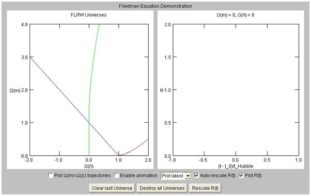
Figure 1.12:Screenshot from the Friedman applet – click here to open a web page containing the applet. |
%3cSUP%3e2%3c/SUP%3e%20=%20(%3cI%3eHR%3c/I%3e%3cIMG%20WIDTH=14%20HEIGHT=28%20ALIGN=MIDDLE%20BORDER=0%20SRC=ansimg4.gif%3e)%3cSUP%3e2%3c/SUP%3e%20=%20(%3cI%3eHR%3c/I%3e)%3cSUP%3e2%3c/SUP%3e%3cIMG%20WIDTH=21%20HEIGHT=35%20ALIGN=MIDDLE%20BORDER=0%20SRC=ansimg5.gif%3e%3c/DIV%3e%3cP%3e%3c/P%3eand%20%3cP%3e%3c/P%3e%3cDIV%20ALIGN=CENTER%3e%3cI%3eV%3c/I%3e%20%3cIMG%20WIDTH=16%20HEIGHT=28%20ALIGN=MIDDLE%20BORDER=0%20SRC=ansimg3.gif%3e%20%3cI%3er%3c/I%3e%3cSUP%3e3%3c/SUP%3e/%3cI%3er%3c/I%3e%20=%20%3cI%3er%3c/I%3e%3cSUP%3e2%3c/SUP%3e%20=%20%3cI%3eR%3c/I%3e%3cSUP%3e2%3c/SUP%3e%3cIMG%20WIDTH=21%20HEIGHT=35%20ALIGN=MIDDLE%20BORDER=0%20SRC=ansimg5.gif%3e.%3c/DIV%3e%3cP%3e%3c/P%3eas%20required.',300,300))
%5e%7b2/4%7d_%7b%7d$%3e%20=%20%3cIMG%20%20WIDTH=54%20HEIGHT=39%20ALIGN=MIDDLE%20BORDER=0%20%20SRC=ansimg34.gif%20%20ALT=$\displaystyle%20\sqrt%7b2%20H_0%20t%7d$%3e%20%3c/DIV%3e%3cP%3e%3c/P%3e%20%20%3cP%3e%20%20',400,300))
The ![]() ,
, ![]() diagram on the left-hand side of
Applet 1.12
is frequently used to show which combinations are currently allowed by the
data. Getting to know this diagram and the various corresponding R(t) curves is a good way to master the
physics of the Friedman equation.
diagram on the left-hand side of
Applet 1.12
is frequently used to show which combinations are currently allowed by the
data. Getting to know this diagram and the various corresponding R(t) curves is a good way to master the
physics of the Friedman equation.
|
6. Current data suggest that |
.%20The%20actual%20value%20you%20clicked%20on%20is%20reported%20in%20the%20title%20of%20the%20right-hand%20panel.%20If%20necessary%20re-click%20until%20you%20are%20pretty%20well%20there%20(due%20to%20the%20finite%20number%20of%20pixels%20you%20will%20get%20either%200.69%20or%200.71%20for%20%3c!--%20MATH%20%20$\Omega_\Lambda$%20%20--%3e%20%3cIMG%20%20WIDTH=25%20HEIGHT=29%20ALIGN=MIDDLE%20BORDER=0%20%20SRC=ansimg35.gif%20%20ALT=$%20\Omega_%7b\Lambda%7d%5e%7b%7d$%3e).%20You%20should%20get%20something%20like%20this:%20%3cIMG%20%20WIDTH=388%20HEIGHT=409%20ALIGN=BOTTOM%20BORDER=0%20%20SRC=screenshot.gif%20%20ALT=71%3e%20%20%3cP%3e%20It%20looks%20like%20%3cI%3eR%3c/I%3e%20=%200%20is%20reached%20just%20to%20the%20left%20of%20-1.0%20on%20the%20bottom%20axis.%20If%20you%20want%20to%20be%20precise%20you%20could%20measure%20the%20distance%20from%20the%20edge%20of%20the%20plot%20to%20the%20tick%20at%20-0.5,%20and%20compare%20this%20to%20the%20gap%20between%20the%200.5%20interval%20tick%20marks.%20In%20this%20way%20I%20find%20%3cI%3eR%3c/I%3e%20=%200%20is%20at%20-0.93,%20i.e.%20the%20start%20(time%20%3cI%3et%3c/I%3e%20=%200)%20is%20at:%20%3c!--%20MATH%20%20\begin%7bdisplaymath%7d%20(t%20-%20t_0)%20/%20t_H%20=%20-0.93%20%20\Rightarrow%20t_0%20%20=%200.93%20t_H%20\end%7bdisplaymath%7d%20%20--%3e%20%3cP%3e%3c/P%3e%20%3cDIV%20ALIGN=CENTER%3e%20(%3cI%3et%3c/I%3e%20-%20%3cI%3et%3c/I%3e%3cSUB%3e0%3c/SUB%3e)/%3cI%3et%3c/I%3e%3cSUB%3eH%3c/SUB%3e%20=%20-%200.93%20%3cIMG%20%20WIDTH=20%20HEIGHT=28%20ALIGN=MIDDLE%20BORDER=0%20%20SRC=ansimg14.gif%20%20ALT=$\displaystyle%20\Rightarrow$%3e%20%3cI%3et%3c/I%3e%3cSUB%3e0%3c/SUB%3e%20=%200.93%3cI%3et%3c/I%3e%3cSUB%3eH%3c/SUB%3e%20%3c/DIV%3e%3cP%3e%3c/P%3e%20In%20other%20words%20the%20present%20age%20of%20the%20Universe%20is%20the%20Hubble%20time%20%20to%20a%20pretty%20good%20approximation.%20Play%20around%20with%20the%20applet%20to%20convince%20yourself%20that%20this%20is%20not%20the%20case%20for%20most%20values%20of%20%3cIMG%20%20WIDTH=16%20HEIGHT=14%20ALIGN=BOTTOM%20BORDER=0%20%20SRC=ansimg12.gif%20%20ALT=$%20\Omega$%3e!%20',500,500))
Although the convention is that ![]() and
and
![]() normally refer to the present time (t0),
it is quite illuminating to see how they change, and Applet 1.12
will show you this. Clicking on the graph shows that nearly all universes start
at the Einstein-de Sitter point with
normally refer to the present time (t0),
it is quite illuminating to see how they change, and Applet 1.12
will show you this. Clicking on the graph shows that nearly all universes start
at the Einstein-de Sitter point with ![]() = 1 and
= 1 and ![]() = 0. This is because if there is a Big Bang (i.e. R
goes to zero at t = 0) then r, hence H, hence rc, all
tend to infinity at time zero. So
= 0. This is because if there is a Big Bang (i.e. R
goes to zero at t = 0) then r, hence H, hence rc, all
tend to infinity at time zero. So ![]() tends to zero, while the matter density tends to the
critical density.
tends to zero, while the matter density tends to the
critical density.
The coloured lines divide the plane into six
regions, in each of which the universe has a rather different character.
The blue line shows where ![]() =
1, i.e. k = 0. Above this line, space is positively curved (and closed),
below it, it is negatively curved, and open in the simplest topology. Evolution
tracks never cross the blue line because k cannot change.
=
1, i.e. k = 0. Above this line, space is positively curved (and closed),
below it, it is negatively curved, and open in the simplest topology. Evolution
tracks never cross the blue line because k cannot change.
The line ![]() = 0 separates universes with negative and positive
cosmological constant. Negative values mean that the universe
always recollapse eventually: the expansion
halts and reverses at a certain point. Since at turnaround H = 0 by
definition, the critical density at turnaround is zero, so the evolution tracks
of universes with turnaround extend out to infinite
= 0 separates universes with negative and positive
cosmological constant. Negative values mean that the universe
always recollapse eventually: the expansion
halts and reverses at a certain point. Since at turnaround H = 0 by
definition, the critical density at turnaround is zero, so the evolution tracks
of universes with turnaround extend out to infinite ![]() on
both axes.
on
both axes.
The green and red lines bound universes with
positive cosmological constants that expand continuously from R = 0 to
infinity. They start from the matter-dominated Einstein-de Sitter point and end
at the ![]() -dominated
de Sitter point
-dominated
de Sitter point ![]() = 0,
= 0, ![]() = 1.
= 1.
The limiting case for an expanding, closed
universe is the loitering universe, first studied by Lemaître.
This corresponds to the curved green and red lines. Loitering universes reach a
point with H = 0 and also zero acceleration, known as the Einstein
solution (which lies at infinity on this graph because the critical density is
zero). Along the green line the Einstein point is in the future, while it is in
the past along the red line. At the Einstein point the repulsive negative
pressure from the cosmological constant exactly balances the gravitational
attraction of mass/energy:
![]() .
.
This is a delicate and unstable balance. If the density is slightly too high, the universe will collapse from the Einstein point, following the green line down to a Big Crunch at the Einstein-de Sitter point. If the density is too low, the expansion takes off and the universe follows the red line to the de Sitter point of total domination by the cosmological constant.
In universes with positive cosmological constant,
but which fall to the left of the green loitering line, the repulsive term is
not enough to prevent recollapse, so they expand from
the Einstein-de Sitter point to a turnaround at infinity, and then recollapse back to a big crunch along the same track. Thus
all the tracks to the left of the green line expand from a big bang and recollapse to a big crunch.
Finally, universes to the right of the red
loitering line have a cosmological constant so large that, projecting the
universe back in time, the expansion turns around in the past; these are the
bounce models, in which the universe collapses from infinity (contracting from
the de Sitter point), bounces (both ![]() s
are infinite at the bounce as H = 0 here, just as at turnaround in
"bang-crunch" universes), and then re-expands, finishing in an
expanding de Sitter phase. Note that the limiting case here is when the
universe collapses from infinity to bounce at exactly the condition for an
Einstein universe, thereby following the red curve away from the de Sitter
point.
s
are infinite at the bounce as H = 0 here, just as at turnaround in
"bang-crunch" universes), and then re-expands, finishing in an
expanding de Sitter phase. Note that the limiting case here is when the
universe collapses from infinity to bounce at exactly the condition for an
Einstein universe, thereby following the red curve away from the de Sitter
point.
1.3.3.4 Open vs. Closed Universes
Cosmologists often talk about open and closed universes. Unfortunately the meaning of these terms has become confused. The founders of modern cosmology, Einstein and Friedman, used them, as we do in this course, in their topological sense. They noted that the simplest topologies associated with positive and negative curvature were closed and open respectively. The possibility of more complex topologies was ignored by their immediate successors, and eventually almost forgotten. At the same time, the cosmological constant became unfashionable, and negative-pressure matter like quintessence was not considered. Without these terms the Friedman equation implies that a negatively curved universe expands forever and a positively curved one recollapses. Eventually cosmologists came to assume that "open" meant negatively curved and forever expanding, while "closed" meant positively curved and with a finite future – the slogan was that "geometry implies destiny".
This slogan is simply false; it is based on a
naive interpretation of the Friedman equation which took far too much for
granted. As we have seen, geometry (i.e. curvature) does not necessarily define
the topology. If there is a cosmological constant, then universes with
negative, zero, or positive curvature can all expand forever or recollapse; which actually happens depends on ![]() and
and ![]() . And, of course, this all assumes that the universe is
genuinely homogeneous and isotropic on the largest scale.
. And, of course, this all assumes that the universe is
genuinely homogeneous and isotropic on the largest scale.
%20from%20the%20ones%20which%20expand%20for%20ever%20(on%20the%20right).%20The%20blue%20and%20green%20lines%20cross%20at%20%3c!--%20MATH%20%20$\Omega_m=1$%20%20--%3e%20%3cIMG%20%20WIDTH=28%20HEIGHT=29%20ALIGN=MIDDLE%20BORDER=0%20%20SRC=ansimg29.gif%20%20ALT=$%20\Omega_%7bm%7d%5e%7b%7d$%3e%20=%201,%20%3c!--%20MATH%20%20$\Omega_\Lambda=0$%20%20--%3e%20%3cIMG%20%20WIDTH=25%20HEIGHT=29%20ALIGN=MIDDLE%20BORDER=0%20%20SRC=ansimg35.gif%20%20ALT=$%20\Omega_%7b\Lambda%7d%5e%7b%7d$%3e%20=%200,%20so%20Euclidean%20universes%20will%20recollapse%20if%20%3c!--%20MATH%20%20$\Omega_\Lambda$%20%20--%3e%20%3cIMG%20%20WIDTH=25%20HEIGHT=29%20ALIGN=MIDDLE%20BORDER=0%20%20SRC=ansimg35.gif%20%20ALT=$%20\Omega_%7b\Lambda%7d%5e%7b%7d$%3e%20is%20negative.%20(If%20it%20is%20zero%20we%20have%20the%20Einstein-de%20Sitter%20universe%20which%20expands%20for%20ever,%20as%20we%20have%20already%20seen).%20%20%3cP%3e%20%20',400,300))
Some cosmologists, rather than admit they have
been confused in the past, now prefer to define "open" and
"closed" to mean "expands forever" and "will
re-collapse". So treat these words with suspicion when you run into them
in popular accounts, textbooks, or research articles.
1.3.4 Horizons
The largest distance that is visible in principle
at a given time is called the particle horizon. There is such a limit
because light travels at a finite speed; thus the particle horizon is the
co-moving distance that light can travel since the beginning of the Universe.
Real photons are obstructed by matter at very early times, so we had better
make clear that for present purposes "light" is assumed to travel
unimpeded.
The particle horizon seems an obvious concept, but
mathematically it can be avoided if the universe expands so fast at the start
that light can travel an infinite co-moving distance. This would only happen in
a universe containing no matter or radiation to decelerate it, so it is not
very realistic! But by the same token, the particle horizon is always further
away that ct0, because the universe expands as the light
travels through it. For instance, for the Einstein-de Sitter case (![]() = 1,
= 1, ![]() = 0), the particle horizon is
= 0), the particle horizon is
![]() .
.
The finite particle horizon is the solution to the
paradox that the sky is dark at night (Olbers'
paradox). See Strobel's notes
for more about this.
At a given time, there may also be a largest
distance that will ever be able to see us. This is called the event
horizon. It is the co-moving distance that light can travel from now until
the end of the Universe.
At first glance we might expect an event horizon
only if the universe re-collapses. Otherwise, it lasts for ever and it is
natural to expect that our light will eventually reach a galaxy at any distance
at all. But in fact, again, the universe may expand too fast. If there is a
positive cosmological constant (which seems to be true for our Universe), then
we eventually reach the exponentially-accelerating de Sitter phase. Exponential
acceleration means that any galaxy will eventually be receding from us faster
than light, so light will never reach it. Photons emitted today will pass many
galaxies, but as they travel and the universe expands, the gulfs between
galaxies widen. Fewer and fewer galaxies are passed with each billion years.
Eventually a last galaxy is reached. Observers there may see a redshifted galaxy yet further away, but this light carries
old news. Since then, that galaxy has accelerated past the speed of light and
our photon will never reach it.
In a universe like ours, with both particle and event horizons, there is a
maximum co-moving distance that a photon can travel in the whole of time, equal
to the sum of the two horizon lengths. Weirdly, if ![]() > 1 and
> 1 and ![]() > 0,
the universe is spatially closed (and so finite in size), lasts forever, and
yet may contain different regions which can never find out about each other's
existence.
> 0,
the universe is spatially closed (and so finite in size), lasts forever, and
yet may contain different regions which can never find out about each other's
existence.
Answers to questions
1. Show that T and V are both proportional to ![]() .
.
Answer to question
We
have:
![]()
and
![]()
as required.
2. Look up "quintessence" in a dictionary. Is it a well-chosen name?
Answer to
question
My dictionary defines quintessence as ''fifth
substance, apart from the four elements, composing the heavenly bodies entirely
& latent in all things''. This is quite appropriate: dark energy does seem
to be the major component of our universe, energetically speaking, and fills
intergalactic space smoothly. In contrast our local environment (e.g. our
galaxy) is dominated by the four substances baryonic matter, cold dark matter,
neutrinos, and radiation, which perhaps are the modern equivalents of earth,
water, air and fire.
3. Calculate
the present value of rc assuming that H0 = 100 km s-1 Mpc-1.
Work out your answer in
(a) kg m-3,
(b) protons m-3,
(c) Galaxies per cubic Mpc (take 1 Galaxy = 1012 solar masses).
Answer to question
![]() .
.
(a) Now H0 = 100 kms-1Mpc-1 = 105 ms-1Mpc-1. Our list of constants gives the length of a parsec in metres, which corresponds to 1 Mpc = 3.086×10²² m, so
H0 = (105/3.086×1022) ms-1m-1 = 3.24×10⁻¹⁸ s-1
in SI units. Putting in the value of G from the constants list, we get
rc(t0) = 1.878×10⁻²⁶ kg m-3.
NB the units of G are N m2 kg-2.
N is
s-2 from H2
and m3 kg-1s-2 from G, giving kgm-3
as advertised.
(b) A proton has mass 1.637×10⁻²⁷ kg, from the constants list. To convert to protons per cubic metre, multiply by (protons per kilogram)= 1/mp, i.e
rc(t0) = 11.47 protons m-3.
(c) If a galaxy has mass 1012 solar masses, this is equal to 1.989×1042kg, using the solar mass from the constants list. 1 cubic Mpc = (3.086×10²²)3 m3, so 1 galaxy (Mpc)-3 is equal to 6.768×10⁻²⁶ kgm-3, and
rc (t0) = 0.3 galaxies (Mpc)-3.
Answer to
question
To get our
equation for H, start with the Friedman Equation
![]()
To find
kc2, substitute the first term on the right hand side with H2![]() , as
derived on the previous line:
, as
derived on the previous line:
![]() .
.
Tidying
up a bit gives - kc2 = H2R2(1
- ![]() ).
This applies at any time, in particular, now:
).
This applies at any time, in particular, now:
- kc2
= H02R02(1
- ![]() ) .
) .
So we
can replace the second term on the right of the Friedman equation with
 .
.
Finally, we
replace the first term on the right with the long expression derived on the
previous line, to give our final formula for the Hubble parameter at any given
value of R, or alternatively of R0/R = (1 + z).
If you're
worried by the previous equation, let's take it more slowly. Starting at the
left, we have
![]() .
.
Cancel H2
on top and bottom:
![]() .
.
Second step
in text is
![]()
which is just the
definition of rc, applied at
time t0.
Third step is
the same for each of the three terms in the
bracket: we'll do it just for the first to cut
down on the algebra. We have
 .
.
Note that ![]() , the value for the present time, as it should be.
, the value for the present time, as it should be.
5. Find the equation for R/R0 when radiation dominates.
Answer to question
When radiation dominates we have n = 4, therefore
 .
.
6. Current data suggest that ![]()
![]() 0.7,
0.7, ![]()
![]() 0.3. Use the applet to plot R(t) for this universe and
hence read off the present age of the universe t0 in terms of the Hubble time tH.
0.3. Use the applet to plot R(t) for this universe and
hence read off the present age of the universe t0 in terms of the Hubble time tH.
Answer to question
Click
on the left-hand panel of the applet roughly at ![]() = 0.3,
= 0.3, ![]() = 0.7
(note that this is on the blue line
= 0.7
(note that this is on the blue line ![]() = 1).
The actual value you clicked on is reported in the title of the right-hand
panel. If necessary re-click until you are pretty well there (due to the finite
number of pixels you will get either 0.69 or 0.71 for
= 1).
The actual value you clicked on is reported in the title of the right-hand
panel. If necessary re-click until you are pretty well there (due to the finite
number of pixels you will get either 0.69 or 0.71 for ![]() ). You should get something like this:
). You should get something like this: 
It looks like R = 0 is reached just to the left of -1.0 on the bottom axis. If you want to be precise you could measure the distance from the edge of the plot to the tick at -0.5, and compare this to the gap between the 0.5 interval tick marks. In this way I find R = 0 is at -0.93, i.e. the start (time t = 0) is at:
(t - t0)/tH = - 0.93 ![]() t0 =
0.93tH
t0 =
0.93tH
In other words the present age of the Universe is
the Hubble time to a pretty good approximation. Play around with the applet to
convince yourself that this is not the case for most values of
![]() !
!
7. What
is the condition on ![]() for a
Euclidean universe to recollapse? (Make reference to
the applet).
for a
Euclidean universe to recollapse? (Make reference to
the applet).
Answer to
question
Euclidean universes correspond to the blue line in
the left-hand panel of the applet. The green line separates universes which
re-collapse (on the left) from the ones which expand for ever (on the right).
The blue and green lines cross at ![]() = 1,
= 1, ![]() = 0, so
Euclidean universes will recollapse if
= 0, so
Euclidean universes will recollapse if ![]() is
negative. (If it is zero we have the Einstein-de Sitter universe which expands
for ever, as we have already seen).
is
negative. (If it is zero we have the Einstein-de Sitter universe which expands
for ever, as we have already seen).