Advanced Tutorial - Polarisation

Data required

This tutorial follows the initial calibration and imaging of e-MERLIN 5-GHz observations of 3C277.1 (see here. For reminders about how to start CASA and run steps in a script, see these tutorials.

• Before beginning, ensure that you have a directory made for this tutorial (e.g., named Polarisation) and that your computer has at least 7GB of space.
• Next, use the link or command below to download the data to that folder:
  • ERIS22_AT4_polarisation.tar.gz (~1.6GB)

  wget https://www.jb.man.ac.uk/DARA/ERIS22/data/ERIS22_AT4_polarisation.tar.gz

• Un-tar the download using tar -xvf ERIS22_AT4_polarisation.tar.gz

You should find the following files in your folder:

1. all_avg_pol.ms - measurement set that has all previous calibration (including self-calibration) applied from the main tutorials.
2. 3C277.1_pol2022.py - script for the polarisation tutorial
3. 1331+3030_IQUV_5GHz.clean.model.tt0 and 1331+3030_IQUV_5GHz.clean.model.tt1 - polarised model for 3C286 (with two frequency terms)

This tutorial script does not have blanks as most parameter settings are unambiguous. Nonetheless, please be sure to read each step in the script before running it. Instead, there are a number of additional steps you could add at the end. There are also optional extra activities highlighted, if you have time.

Table of contents

Important: The numbers in brackets respond to the steps in the accompanying python script.

1. Prepare data set (0-1)
2. Set models and inspect data (2-5)
3. Derive corrections for cross-hand delay, leakage, polarisation angle and apply (6-9)
4. Image 3C286 in full polarisation and plot the polarised image (10-11)
5. Apply calibration and image target in full polarisation, plot polarised image (12,13)
6. Additional activities

1. Prepare the data set

← back to top

Some notes on the measurement set we are using, all_avg_pol.ms. This was made from all_avg.ms containing 3C277.1 and its calibrators, as from the total intensity calibration script, which was also flagged. All the calibration has been applied to the calibration sources. For the target, the self-calibration solutions were also applied while it was still in the data set with all the calibrators. The calibrated data are then split out, so that the $\texttt{CORRECTED_DATA}$ column in all_avg.ms becomes the $\texttt{DATA}$ column in all_avg_pol.ms

Step 0

Do not run this step, it is there for information only.

Step 1

This step lists the information on the measurement set. all_avg_pol.ms.listobs should contain,

================================================================================
           MeasurementSet Name:  /raid/amsr/3C277.1/Polarisation/all_avg_pol.ms      MS Version 2
================================================================================
   Observer: TS8004     Project: TS8004  
Observation: e-MERLIN
Data records: 940748       Total elapsed time = 79789.8 seconds
   Observed from   01-Aug-2019/23:20:10.5   to   02-Aug-2019/21:30:00.3 (UTC)

   ObservationID = 0         ArrayID = 0
  Date        Timerange (UTC)          Scan  FldId FieldName          nRows     SpwIds   Average Interval(s)    ScanIntent
  01-Aug-2019/23:20:10.5 - 00:00:00.2     1      3 0319+4130          35820  [0,1,2,3]  [4, 4, 4, 4] 
  02-Aug-2019/00:00:04.0 - 00:00:07.0     2      2 1302+5748             60  [0,1,2,3]  [3, 3, 3, 3]
......... 
              21:00:03.0 - 21:30:00.3   368      0 1331+3030          10768  [0,1,2,3]  [4, 4, 4, 4] 
           (nRows = Total number of rows per scan) 
Fields: 4
  ID   Code Name                RA               Decl           Epoch        nRows
  0    ACAL 1331+3030           13:31:08.287300 +30.30.32.95900 J2000        46256
  1         1252+5634           12:52:26.285900 +56.34.19.48800 J2000       560340
  2         1302+5748           13:02:52.465277 +57.48.37.60932 J2000       242296
  3    CAL  0319+4130           03:19:48.160110 +41.30.42.10330 J2000        91856
Spectral Windows:  (4 unique spectral windows and 1 unique polarization setups)
  SpwID  Name   #Chans   Frame   Ch0(MHz)  ChanWid(kHz)  TotBW(kHz) CtrFreq(MHz)  Corrs          
  0      none      64    GEO    4817.000      2000.000    128000.0   4880.0000   RR  RL  LR  LL
  1      none      64    GEO    4945.000      2000.000    128000.0   5008.0000   RR  RL  LR  LL
  2      none      64    GEO    5073.000      2000.000    128000.0   5136.0000   RR  RL  LR  LL
  3      none      64    GEO    5201.000      2000.000    128000.0   5264.0000   RR  RL  LR  LL

2. Set models and inspect data

← back to top

We split out the corrected column to make further calibration more convenient (why?) but this means that we have to re-insert models for the calibrators and in fact use a new, polarised model for 3C286 (1331+3030).

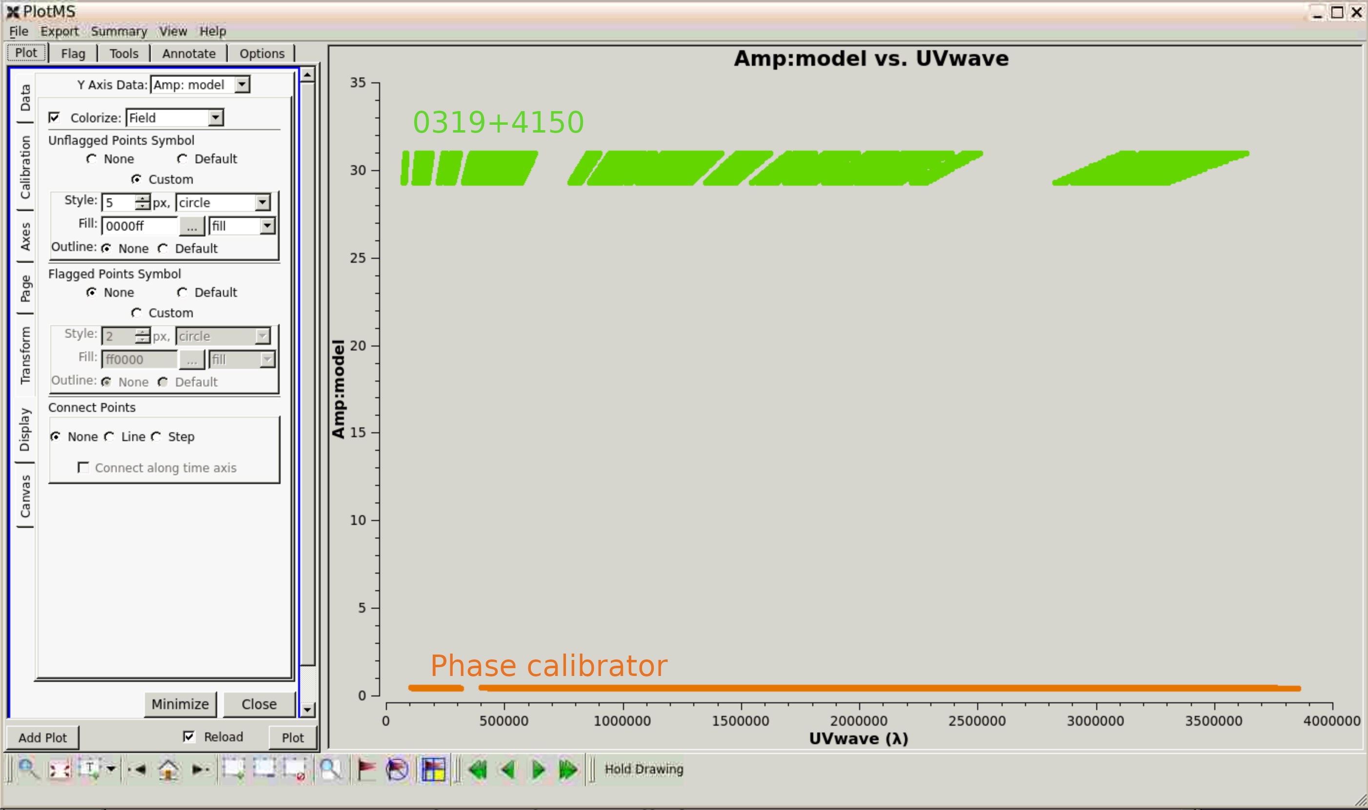
Step 2

Uses the flux density provided for 0319+4130 and the flux density which you previously derived for the phase reference 1302+5748. Tip: If you need to find a previously-set flux density, you can do it like this in CASA:

listhistory(vis = 'all_avg_pol.ms')

Note: For both 0319+4130 and 1302+5748, we set only the Stokes $I$ flux (see above, where fluxdensity = [0.449, 0.0, 0.0, 0.0] (you can also check for 0319+4130). These values are for Stokes [ $I$, $Q$, $U$, $V$]. The $Q$, $U$, $V$ are zero for different reasons: for the phase reference 1302+5748 we do not know the polarised flux density. For 0319+4130 (3C84) we do know - that it is indeed zero at this frequency range and resolution!

The flux density for 1331+3030 (3C286) is set by using a model derived from imaging, since it is both polarised and resolved. The task ft Fourier transforms the clean components and inserts them in the model column of the MS. You can check that 1331+3030_IQUV_5GHz.clean.model.tt0 has 4 Stokes planes either with task imhead or in the viewer.

Question: In ft, why do we use .tt0 and .tt1 images and nterms=2?

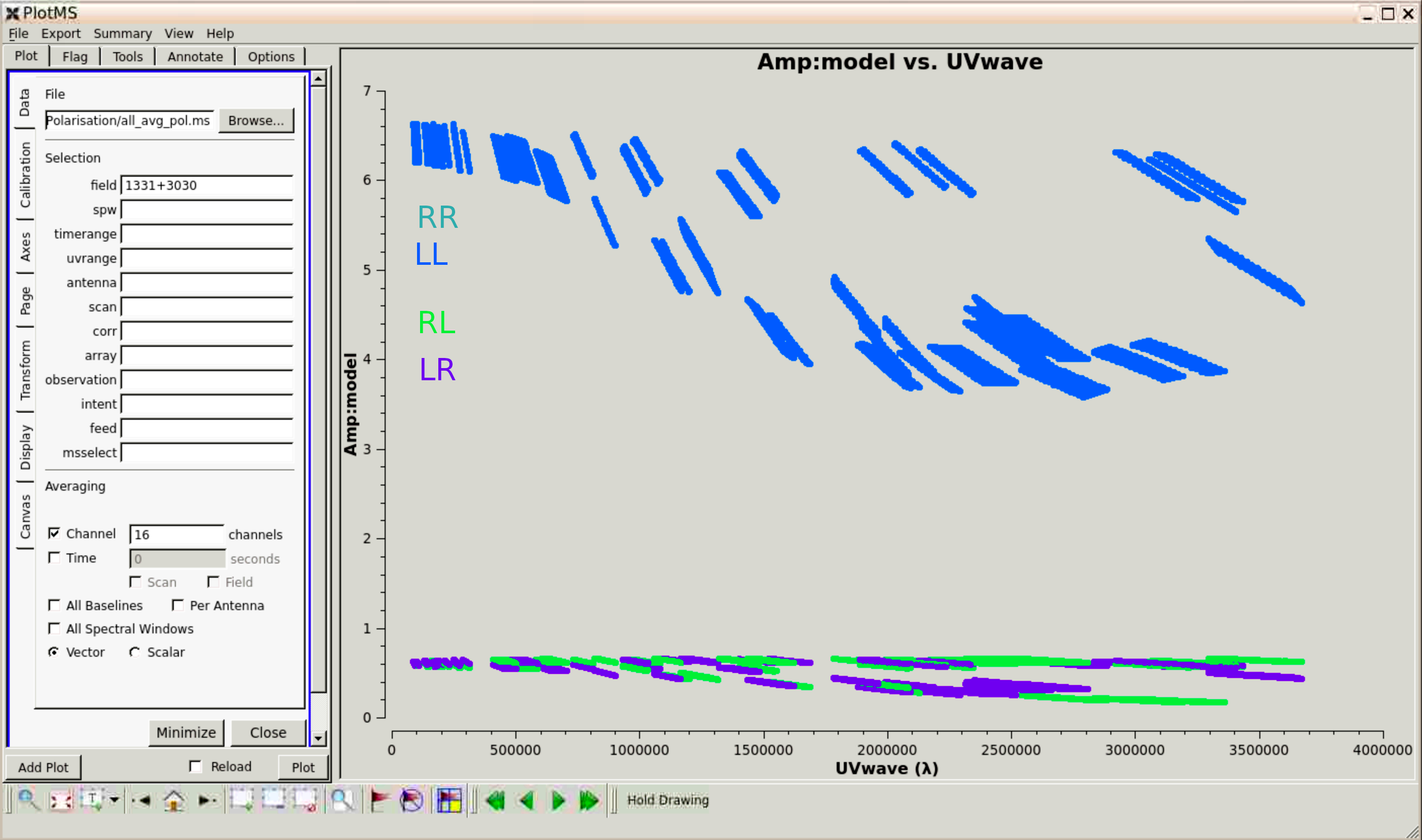
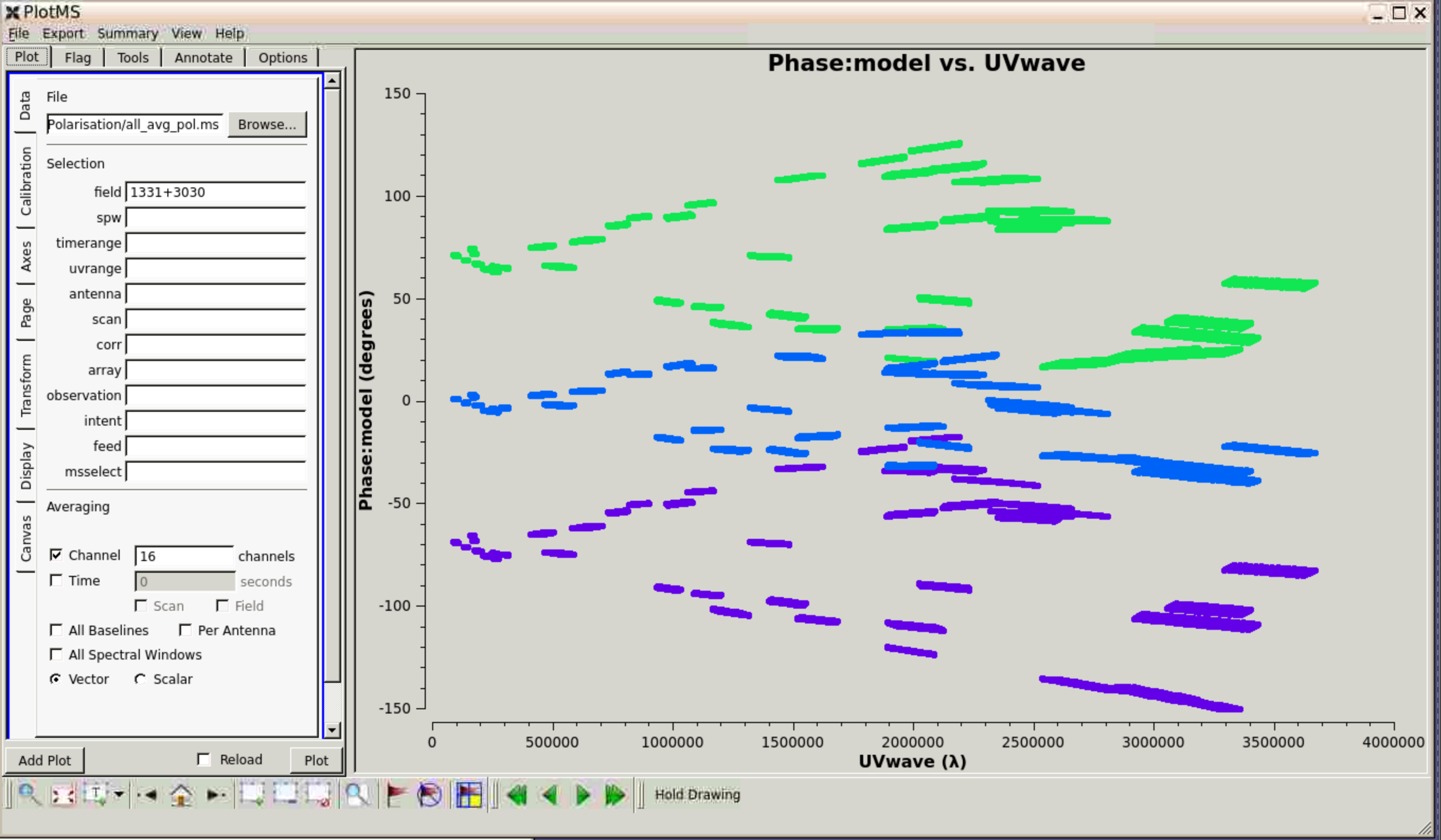
Step 3

This step plots the model amplitude against uv distance for 3C286 so that you can see that it is about $11\%$ polarised. Interactively or by adding to the script, plot phase as well. Note the values of RL and LR (green and purple) at the shortest uv distance, $\pm66$ degrees, or twice the map linear polarisation position angle (see previous talk). You might find the overall shape easier to understand if you plot phase against time and iterate through the baselines. You also could plot the models for the other calibration sources (they should be boring)

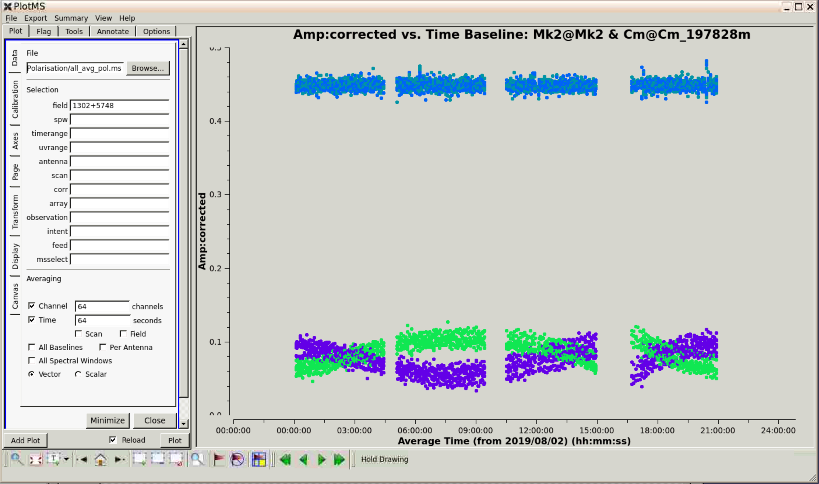
Step 4

This step plots the phase reference $\texttt{DATA}$ phase against time to show parallactic angle rotation.

Questions: This is for a long baseline, what would you expect it to look like on a shorter baseline? Check. What would you expect a similar plot for the target to show (if it was bright enough)?

Step 5

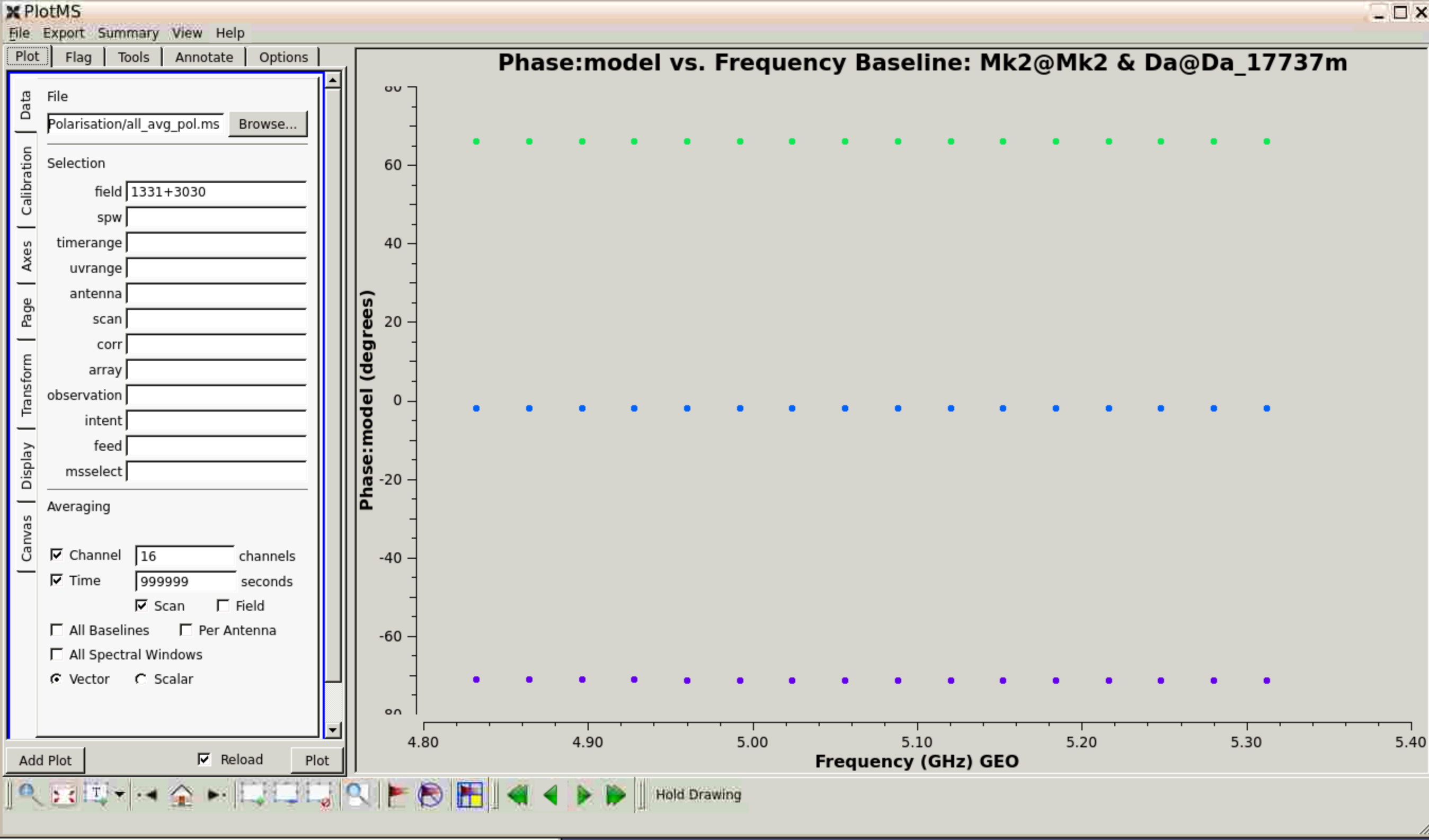
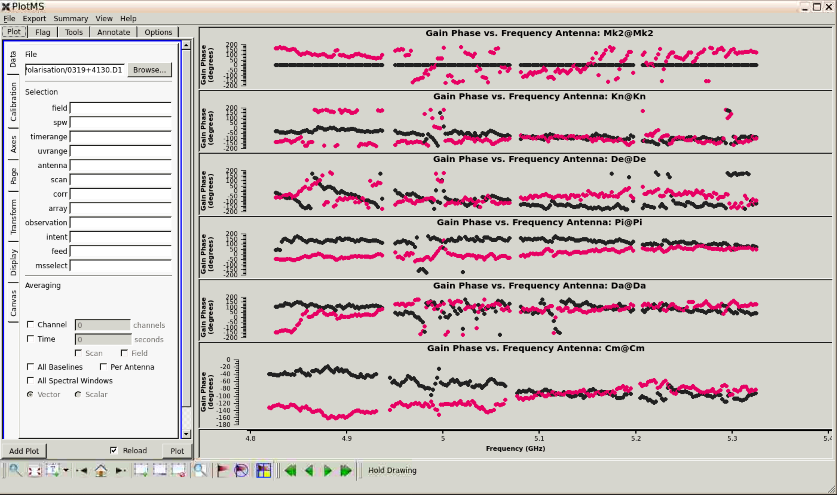
This step plots the uncorrected cross-hand delay, that is, the slope of phase with frequency.

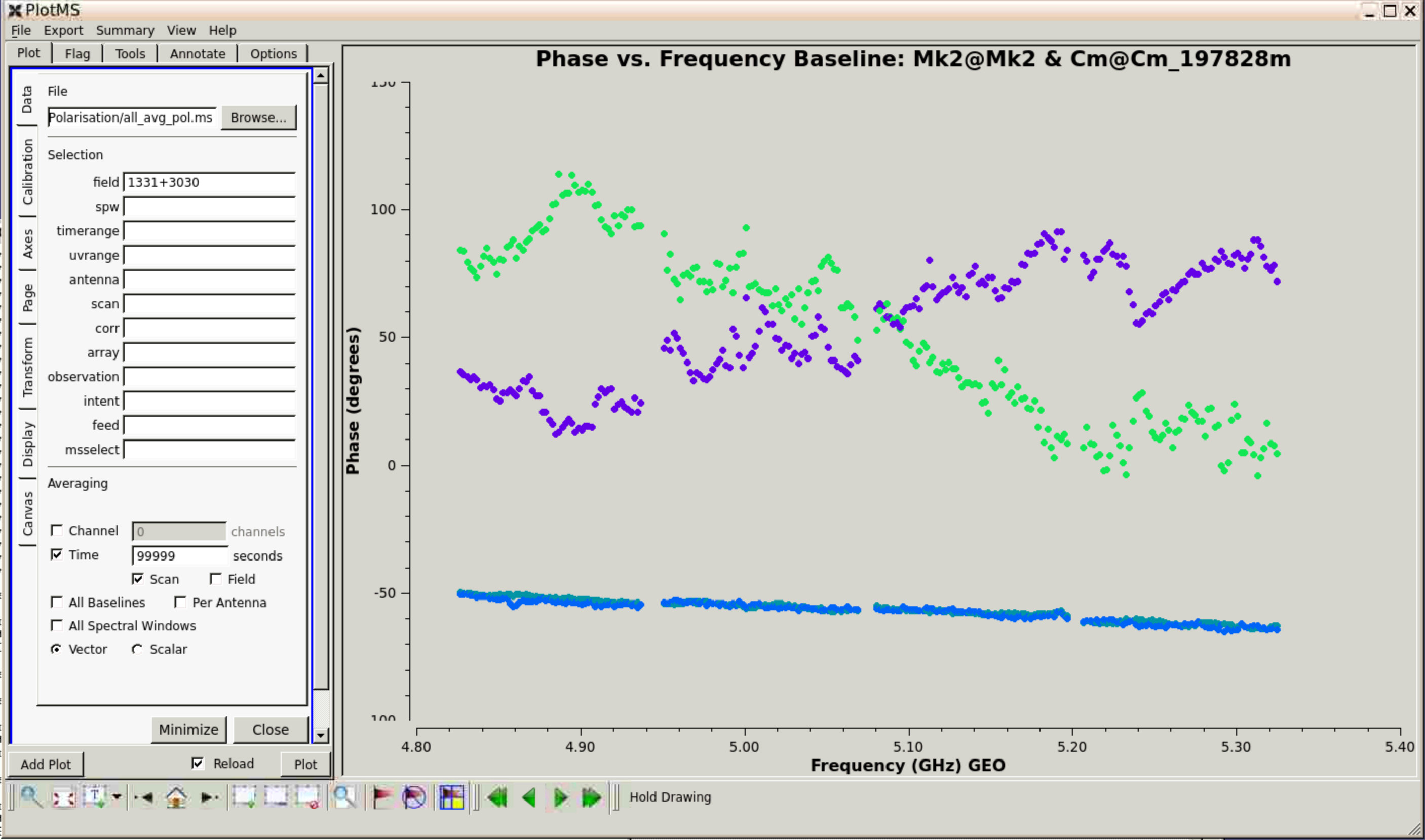
Below, this is compared with the model phase - so we can be sure that the slope on the actual data is due to instrumental errors. Recall that in deriving the initial calibration delay and bandpass corrections, the phase of Mk2 was held constant, but the errors in its cross-hands were thus never corrected and propagate to all the other antennas. Hence the cross-hand delay correction should be the same for all antennas. Note that the model was observed at a different time from these data.

3. Derive corrections for cross-hand delay, leakage, polarisation angle and apply

← back to top

Step 6

In this step we derive the cross-hand delay correction using 1331+3030 as it has fairly strong (~0.6 Jy) emission in the cross hands. As an instrumental correction, it is expected to be constant in time over the observing session, and as it is mainly due to the reference antenna it should be constant for all antennas, hence solint='inf', combine='scan'.

Question:From the Mk2-Cm uncorrected delay, what do you expect to be the magnitude of the correction in nanoseconds?

Check this from the plot; the casalogger will give the plot range, too:

2022-09-09 16:28:21 INFO PlotMS	Delay:data: -0.451982 to 0 (unflagged); (no flagged data)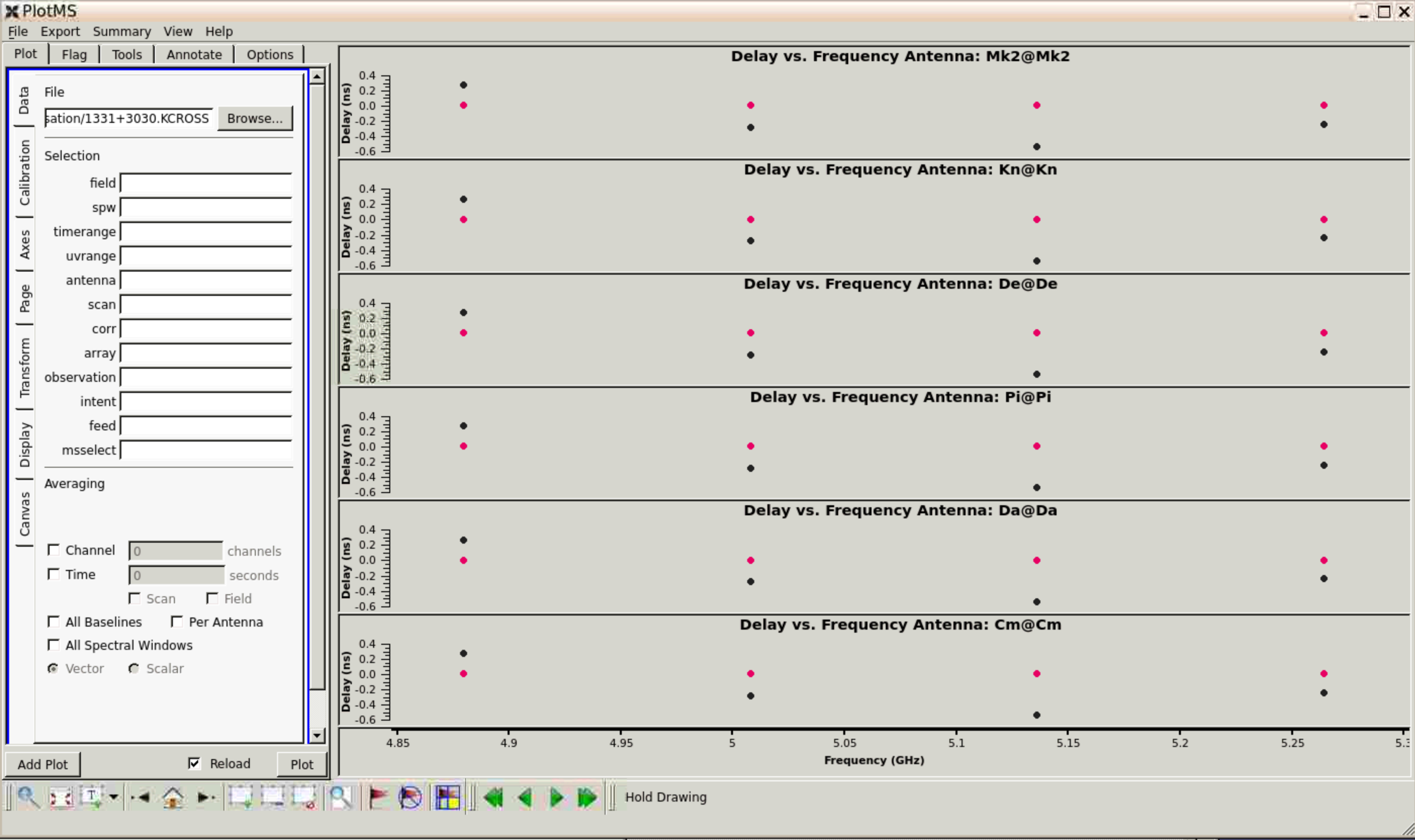

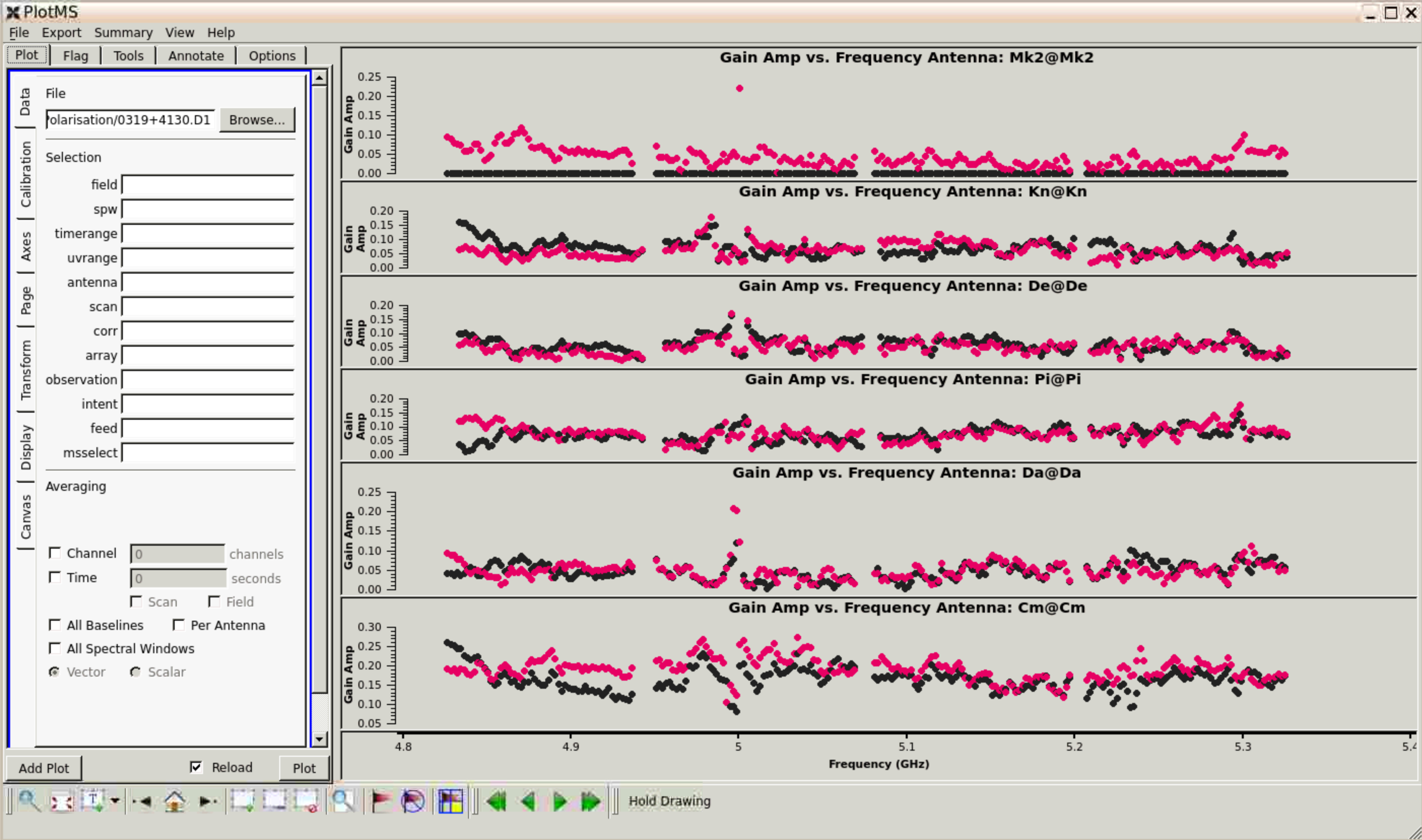
Step 7

Step derives the leakage corrections, that is, the leakage of receiver signal between the hands of polarisation due to imperfections in the waveguides, electronics etc. As noted, this is simple as we have a calibration source, 3C84, which is known to be unpolarised.

Question:When applying 1331+3030.KCROSS, we use spwmap=[0,0,0,0]. Can you work out why?

polcal(vis='all_avg_pol.ms',
         caltable= '0319+4130.D1',
         field='0319+4130',
         minblperant=2,
         minsnr=3,       
         refant=antref,
         poltype='Df',  # Leakage is frequency-dependent
         solint='inf',  # but constant in time for a given receiver
         combine='scan',
         preavg=120.0,  # pre-averaging time (s) (with ~constant parallactic angle)
         gaintable=['1331+3030.KCROSS'],
         spwmap=[0,0,0,0],
         interp='nearest' )

The pre-averaging is not strictly needed here but does no harm, see the extra activities at the end for its use. Since we averaged all spectral windows in deriving 1331+3030.KCROSS, there is only one spw entry in that table, so we use the spwmap parameter here to apply the one correction to all four spw present.
The leakage is pretty messy but should not exceed ~20% in amplitude at these frequencies.

Step 8

The final correction, derived in Step 8, is for polarisation angle $\chi$, which is derived from the R-L visibility phase offset (see talks). $\chi = 0.5\arctan(U/Q)$. 3C286 has a well-known polarisation angle which is almost constant at 33 degrees (hence the $\pm$66 degree relationship between RL and LR). Look at the script and check you understand the parameter settings.

At around 5 GHz, the errors are constant in time for the duration of these observations, but see Michiel Brentjen's talk for the issues at lower frequencies.

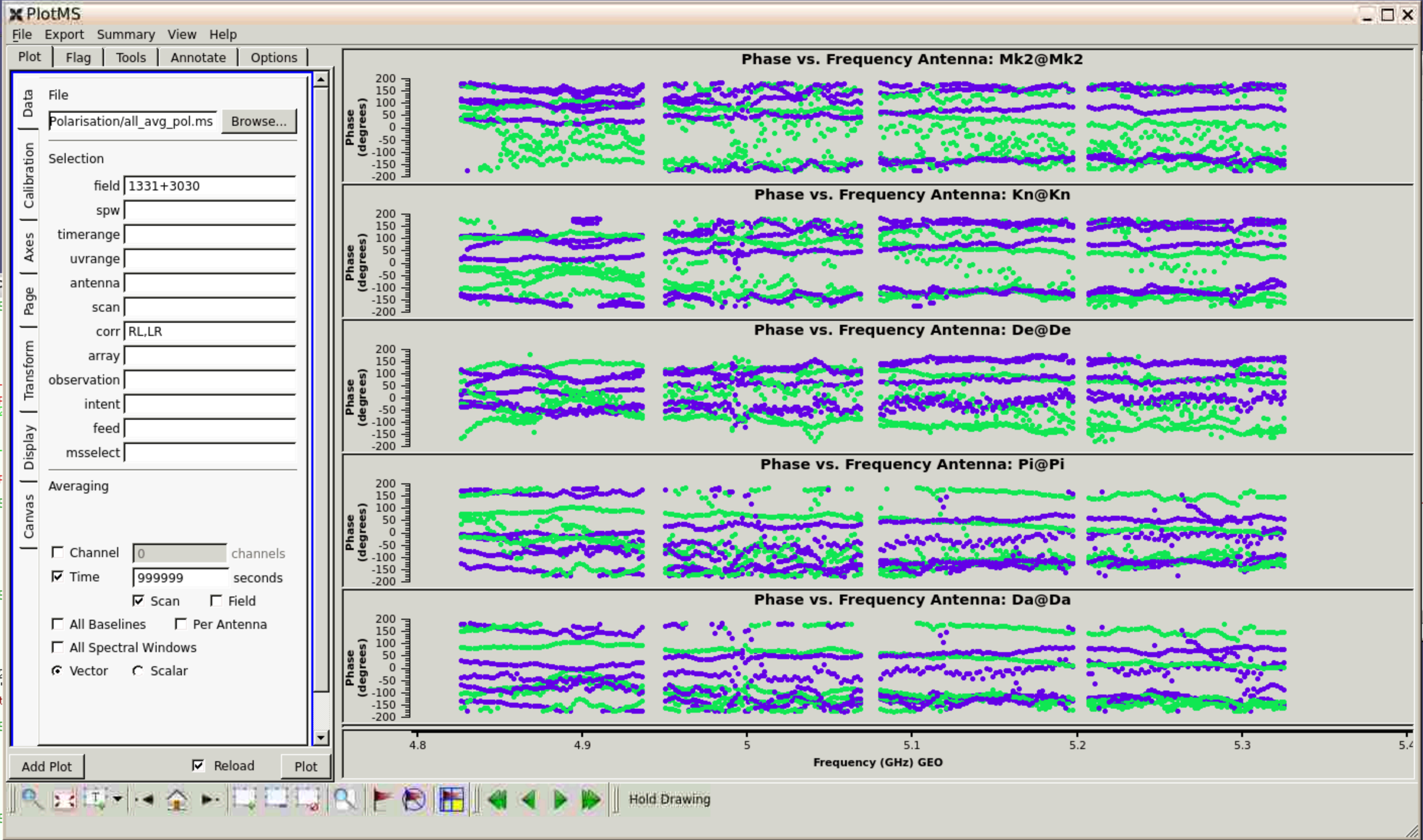
Step 9

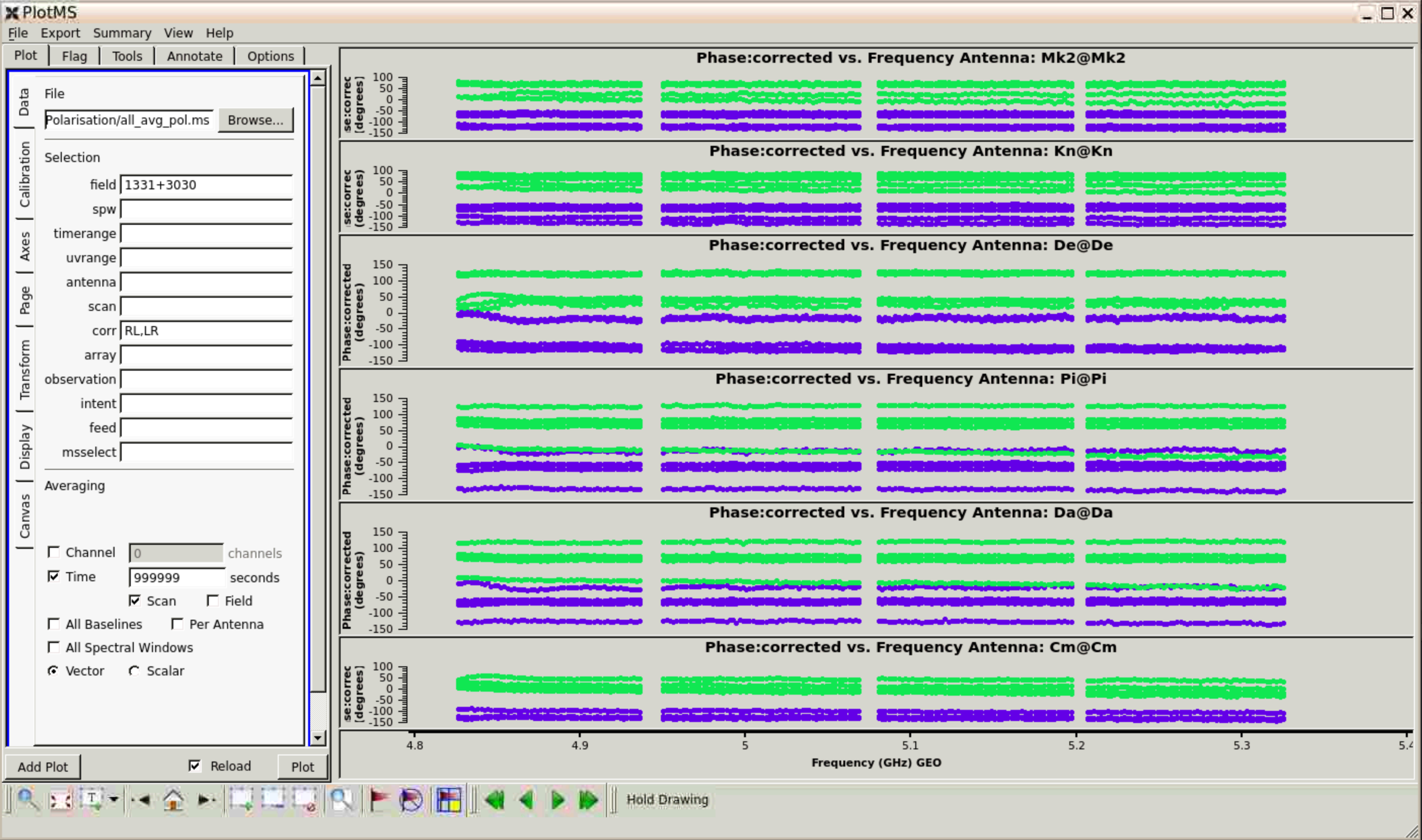
Step 9 applies the polarisation corrections to 3C286 and 3C84 and plots the corrected visibilities for 3C286, showing the improvements before and after. Below is the uncorrected delay.

And the corrected delay:

4. Image 3C286 in full polarisation and plot the polarised image

← back to top

Step 10

Before looking at Step 10, refresh your memory from the Imaging tutorial and think about what parameters you need to make a full polarisation image.

tclean(vis='all_avg_pol.ms',
         field='1331+3030',
         imagename='1331+3030.clean',
         stokes='IQUV',
         restoringbeam='common',
         cell='0.005arcsec',
         imsize=200,
         uvtaper='0.07arcsec',
         interactive=True,
         niter=200)

Some notes on these parameters:

• The obvious one is stokes='IQUV'.
• restoringbeam='common' is used because, if different Stokes parameters have been flagged differently, or even just due to the different orientations of the feeds, very slightly different beams may be fitted for the different Stokes. Some later analysis tasks cannot cope with this, so we force the beam to be the same for each Stokes plane. (This is also worth remembering for spectral cubes as long as the frequency range is not so great that you need a different beam).
• uvtaper='0.07arcsec' is used because 3C286 has a bright core but also weak and very extended emission which is resolved out by e-MERLIN, especially as the observation is very short. The effect of this taper is to apply a Gaussian weighting to the visibility data such that baseline lengths contributing 0.07 arcsec resolution (i.e., approximately the average of the naturally fitted beam) have half-weight, longer baselines have less weight etc. and the resulting beam is more circular and artefacts are reduced.

When imaging remember to mask 'all polarisations' as shown below,

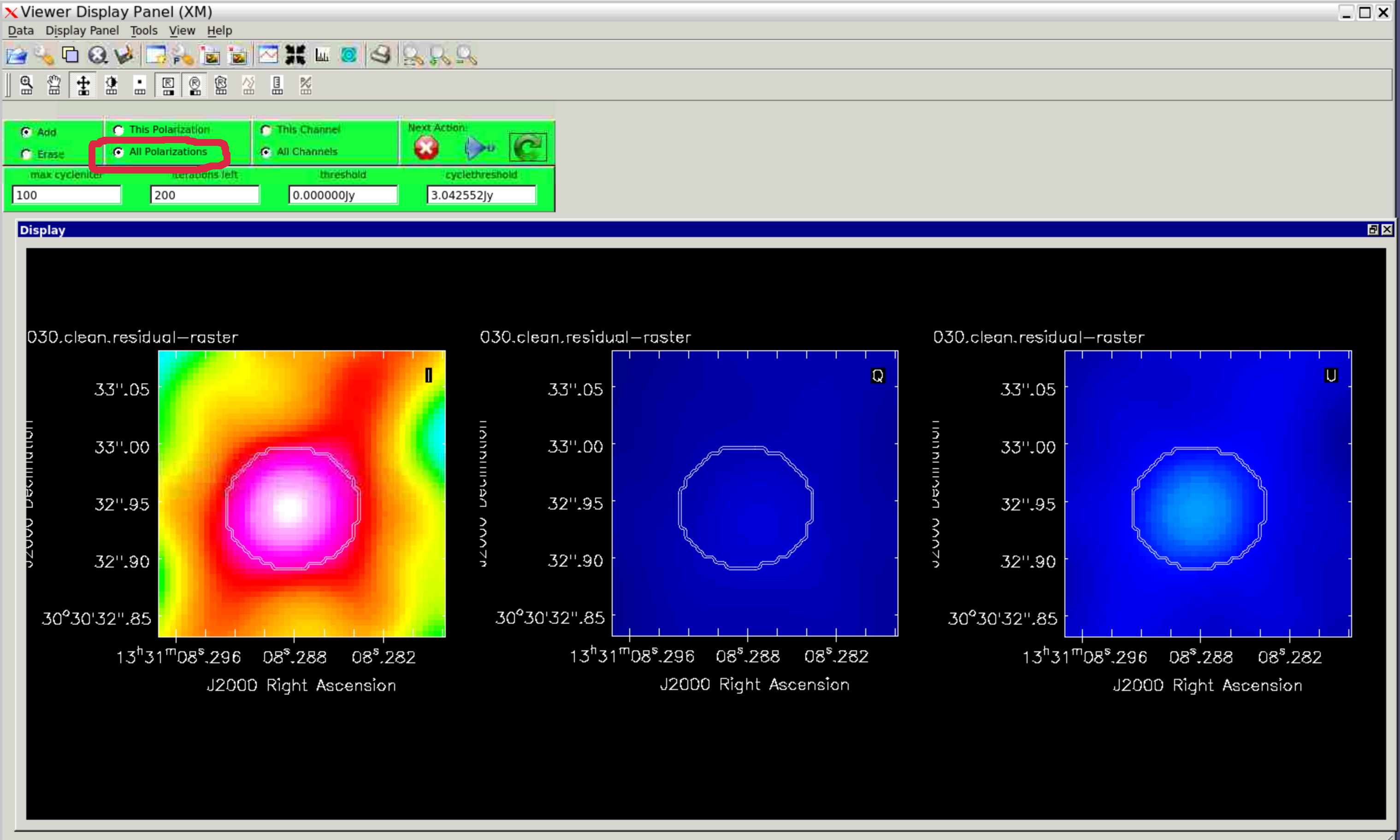
At first you will see in the logger that clean components are only found for Stokes $I$, but $Q$ and $U$ should start to be cleaned as the threshold (as a fraction of the residuals) decreases.

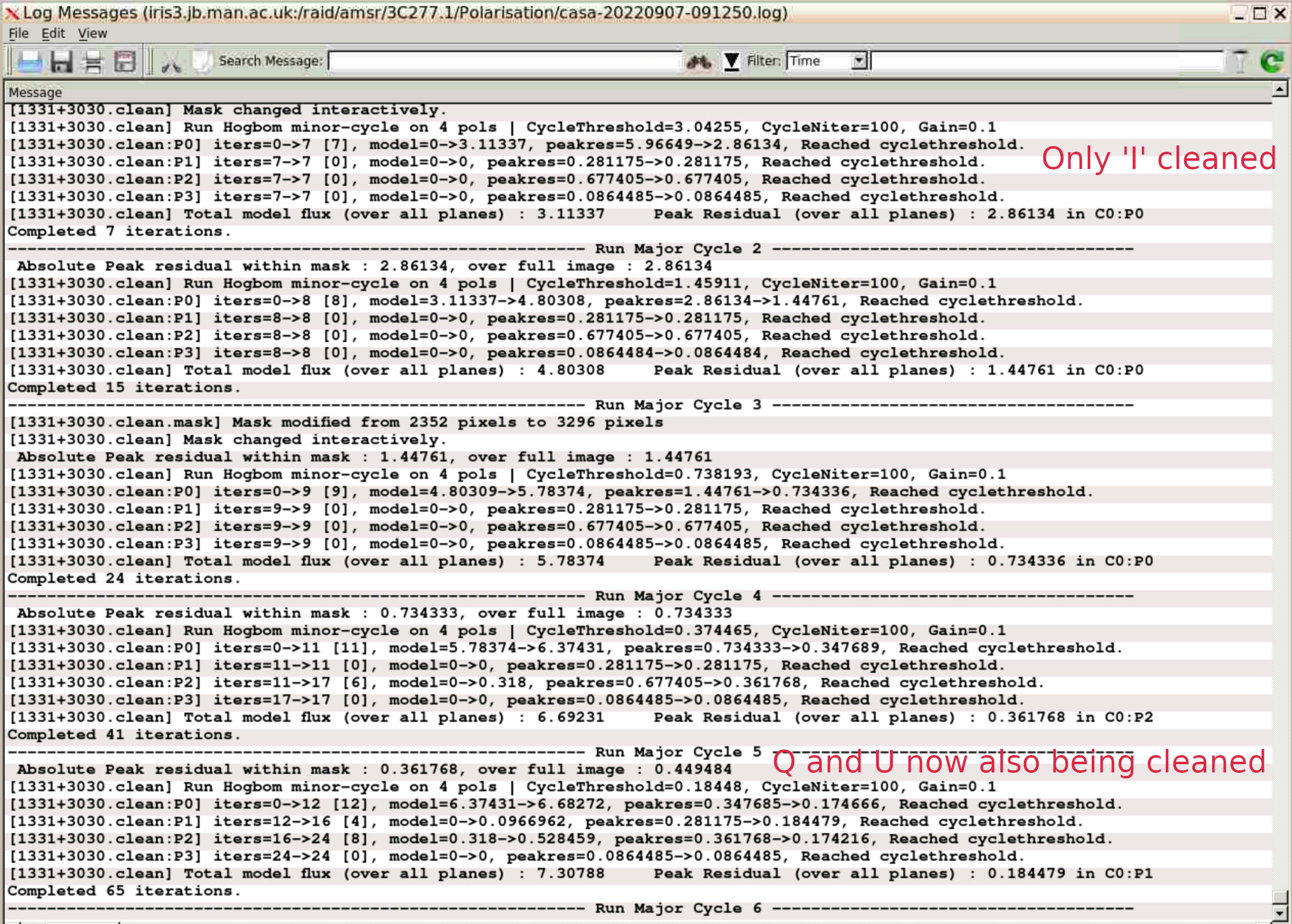
Keep cleaning until you get to the residuals that look like noise (see below) and stop cleaning

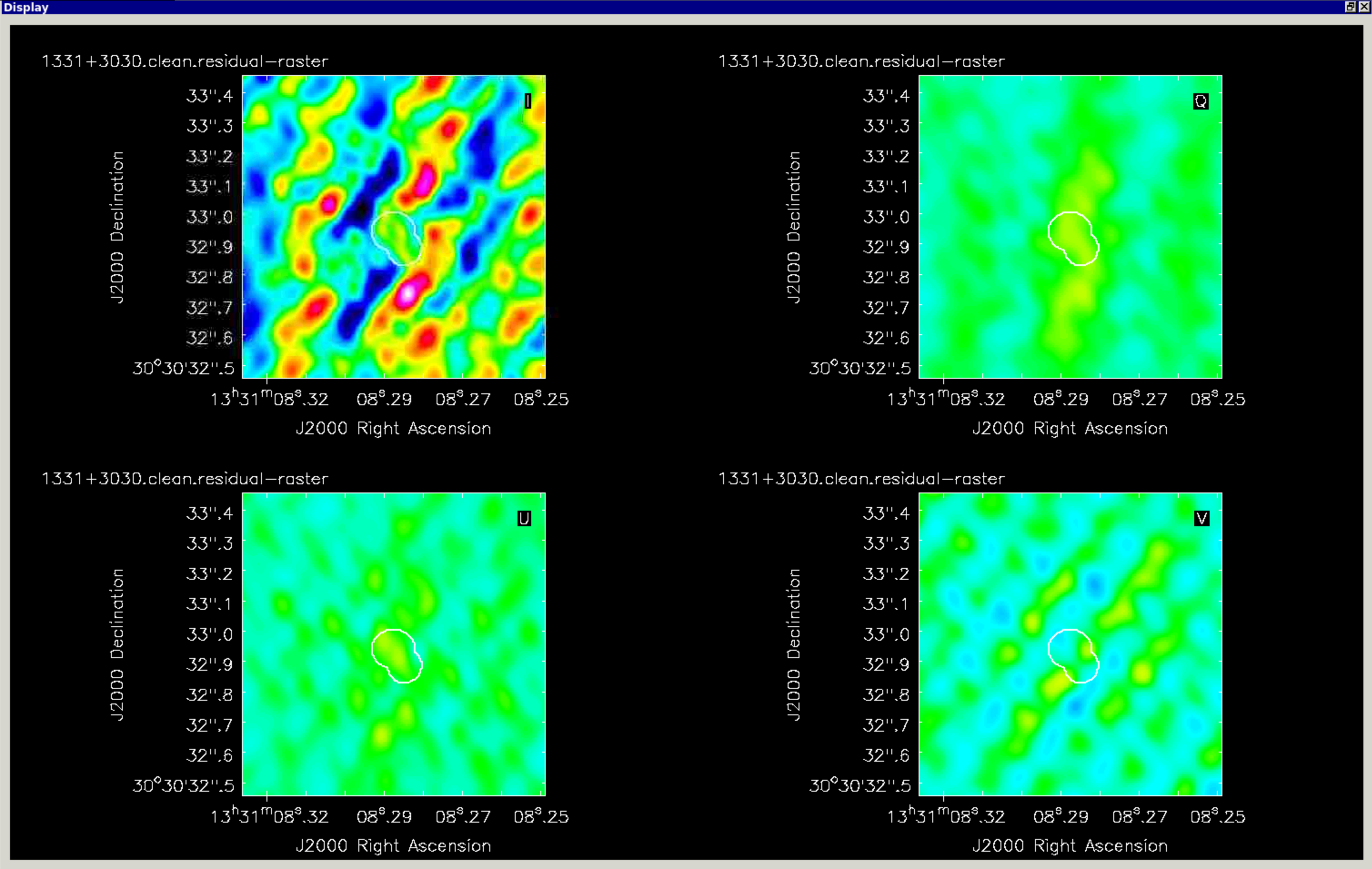
This should make images that look like those below

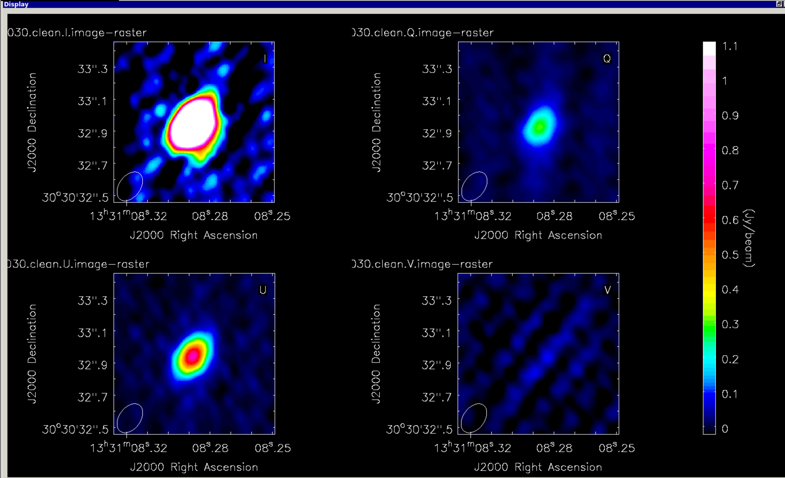
This step also uses task immath to split out the planes of the cube, and then imstat to measure the peak and rms of each image. The boxes are chosen to cover the centre of the image for the peak, and to exclude it for the rms. Values are printed out. I got these, but you might get different values depending on masking and how deeply you cleaned.

# 1331+3030.clean.I.image rms  56.080 mJy
# 1331+3030.clean.I.image peak 6260.000 mJy/bm
# 1331+3030.clean.Q.image rms   9.013 mJy
# 1331+3030.clean.Q.image peak 297.321 mJy/bm
# 1331+3030.clean.U.image rms   7.843 mJy
# 1331+3030.clean.U.image peak 710.796 mJy/bm
# 1331+3030.clean.V.image rms  16.035 mJy
# 1331+3030.clean.V.image peak  86.381 mJy/bm

Question: Why is the rms lower in $Q$ and $U$?

Note that $V$ should be zero, or at least compatible with noise; here it is about $5\sigma$ which shows that there is residual leakage, but at a similar level to the $I$ noise.

Step 11

In this step, we will make polarisation products. First, polarised intensity $P$,

Question: What is the operation on the images used to make linear polarised intensity?

immath(imagename ='1331+3030.clean.image',
         mode='lpoli',
         sigma = '0.01Jy/beam',
         outfile='1331+3030.clean.poli')

The task forms $P = \sqrt{Q^2+U^2}$. However, such an image is entirely positive, but the noise in the original interferometry images is both positive and negative. Hence, the calculated polarised intensity will be slightly too high unless it is debiased. The sigma parameter should be approximately the expected noise in $P$. The exact relationship is more complicated, see the talk and references.

You can predict the error in the Poli ($P$) map by propagation of error, and use this to check or change the value set in the script for sigma in CASA:

from math import *
P = sqrt(Q**2+U**2) 
Q = 297.321
U = 710.796
errQ= 9.013
errU= 7.843
errP=(sqrt(U**2*errU**2+Q**2*errQ**2))/P

Next, polarisation angle map Pola ($\chi$). Here, polithresh is the limit of believable linear polarisation, about 3 $\times$ noise, check/change as needed.

immath(imagename ='1331+3030.clean.image',
         mode='pola',
         polithresh='0.03Jy/beam',
         outfile='1331+3030.clean.pola')

You can calculate the approximate polarisation angle at the peak in CASA:

POLA = 0.5*degrees(atan2(U, Q))

Nb: If you really want to check the error in $\arctan$, it is,

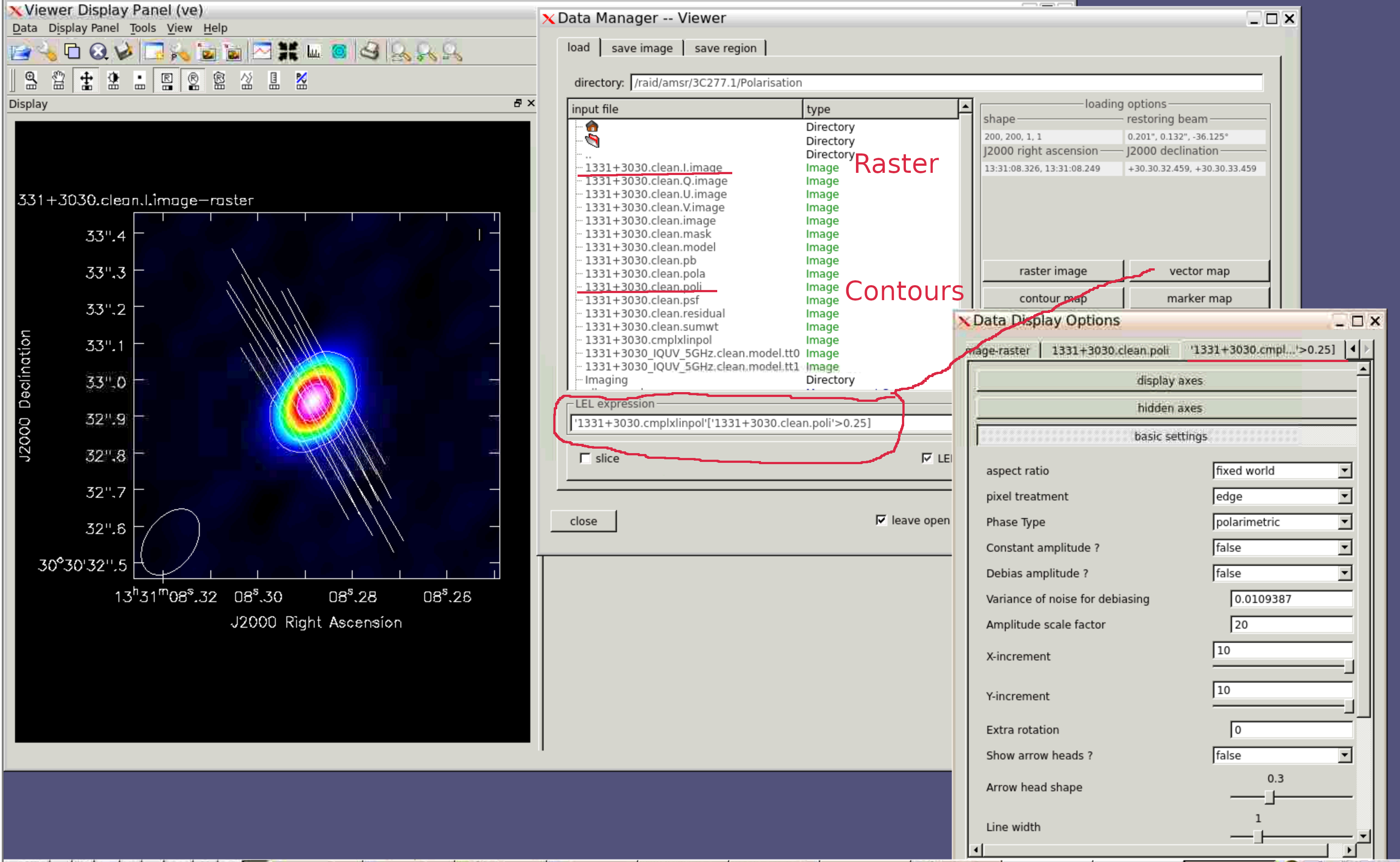
errPOLA=degrees(0.5*sqrt((U**2*errQ**2 + Q**2*errU**2)/(U**2+Q**2)**2))

• 1331+3030.clean.I.image as raster
• 1331+3030.clean.poli as contour
• 1331+3030.clean.pola as vector

Even better, it is possible to display the vectors' lengths proportional to the polarised intensity. In Step 11, this is done by making an image thus:

po.open('1331+3030.clean.image')   # this is the 4-plane IQUV image
po.complexlinpol('1331+3030.cmplxlinpol')
po.close()

You can find more about the use of the imagepol tool in https://casadocs.readthedocs.io/en/stable/notebooks/image_analysis.html and https://casa.nrao.edu/docs/casaref/imagepol-Tool.html

Then, as before, open the total intensity and Poli images, but then, instead of clicking on an image, just enter the following in the LEL box as shown below:

'1331+3030.cmplxlinpol'['1331+3030.clean.poli'>0.25]

This means, open the cmplxlinpol image where the Poli image exceeds 0.25 Jy (change the threshold as wanted).

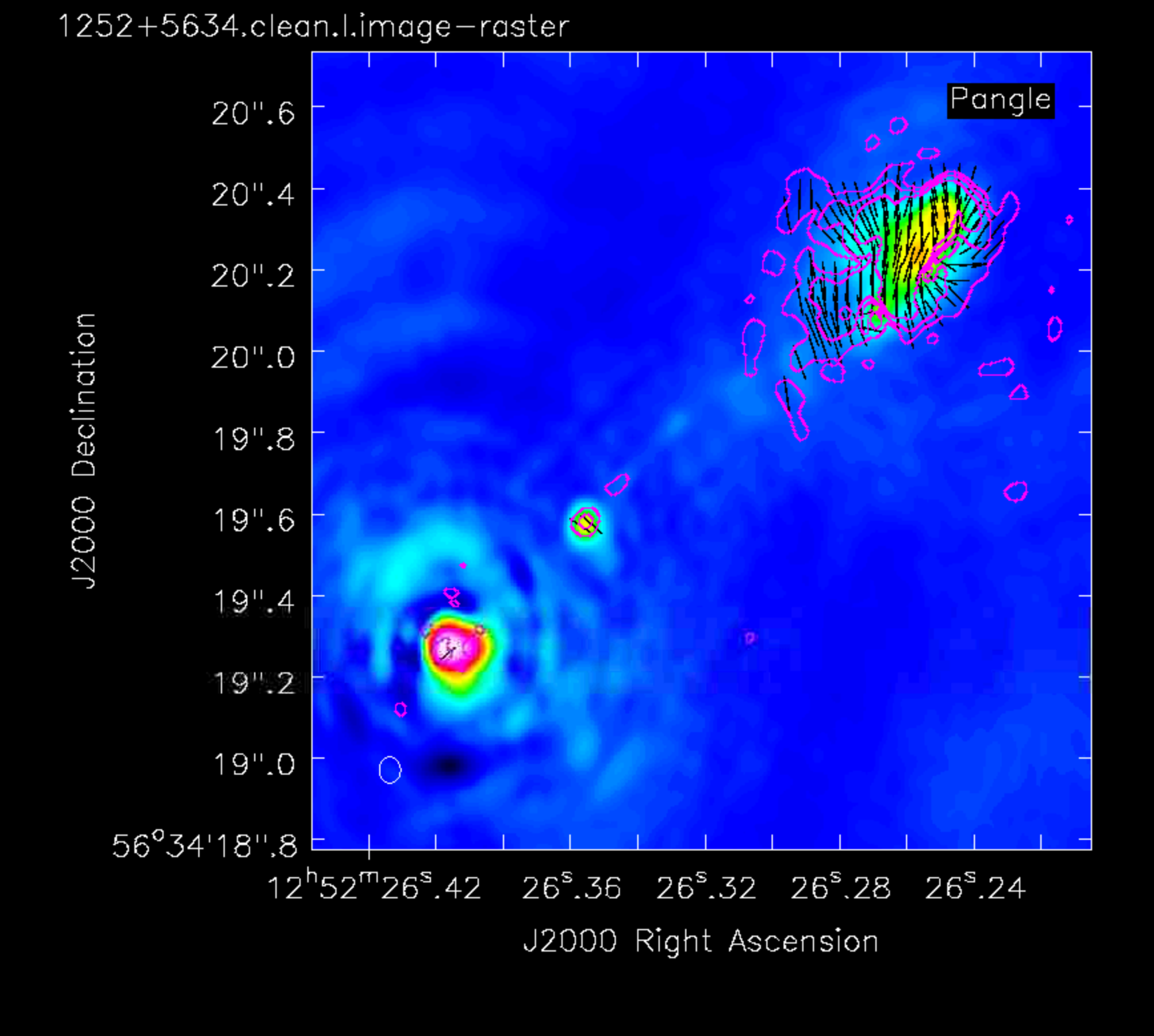
5. Apply calibration, image target in full polarisation and plot the polarised image

← back to top

These are the same procedures as for calibrating and imaging 3C286, but you will need more clean iterations and masking (don't forget, all polarisations!) and different thresholds.

The final image will look something like this:

6. Additional activities

← back to top

Suggestions for further work:

A. These data:

1. Estimate the errors in the polarisation images of 3C277.1, from the images and/or analytically
2. Experiment with the different weightings and imaging parameters as at the end of the imaging and self-calibration tutorials, but in full polarisation.
3. Image 3C84 in polarisation and use it to estimate residual leakage error
4. Rewrite step 7 to use the phase calibrator as a leakage calibrator. In this case, we do not know the source polarisation in advance, but the observations are more than 3 hr. Thus , use poltype = 'D+QU' to solve simultaneously for source polarisation and leakage, using the property that the source polarisation angle will rotate with the sky but the leakage will be fixed to the telescope orientation. This means that, given a long enough observation, the (analytically known) parallactic angle rotation can be used to separate these properties. Then apply the calibration and image the phase reference in polarisation.

B. Look at the polarisation CASA guides:

1. VLA (similar to e-MERLIN, but also outlines Rotation Measure analysis)
2. ALMA (linearly polarised feeds)