2.1 Equipment
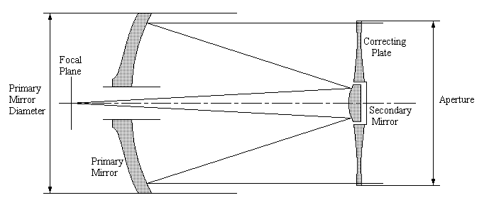
The main feature of the observatory is a 10-inch LX200 Meade Schmidt-Cassegrain telescope. A schematic of this is shown in Figure 2.1.
The telescope consists of a 2-sided aspherical correcting plate, an oversize spherical primary mirror and an aspherical secondary mirror that bring the image to a focus in the focal plane. The focal length, F = 2500mm and the telescope aperture, D = 254mm, give the telescope an f ratio of f/10. The spherical mirror is oversize and therefore bigger than the aperture at 263.525mm. This results in a wider fully illuminated field of view than is possible with a standard primary mirror.
The telescope is equatorially mounted and fully steerable at four speeds along both the right ascension and declination axes. The steering is done via a handheld panel connected to the telescope. This allows objects, once identified with the naked eye to be lined up in the eyepiece. The image can then be focussed manually.
The theoretical resolution of a telescope due to diffraction,2
The CCD is a SBIG ST-6 CCD Camera that can be cooled to 40 50 0C below the ambient temperature. It consists of an array of 375 ´ 242 pixels,3 each 23 ´ 27 m m3 in size. Each pixel saturates at 65,535 counts,4 but it is advisable not to approach this value as the CCD response can become non-linear. An upper limit of 10,000 counts was used in the course of this project. The practical spectral region in which the CCD can be used is between 3700 Å in the near UV and 9000 Å in the near IR. The total dimensions of the CCD are 8.63 ´ 6.53 mm, which can be used to calculate the theoretical field of view.
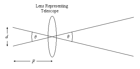
Using the small angle approximation, the angular size on the sky (in radians), q i, of each dimension, di is given by
The spectrometer used in the observatory is a n -View fibre optic spectrometer, a schematic of which is shown in figure 2.3.
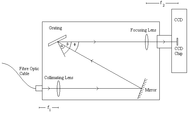
The spectrometer is based on a reflection grating and two f/2 achromatic lenses, which collimate and focus the incident light beam onto the CCD chip. The angle of the reflection grating can be changed using a micrometer. Due to the grating equation,5
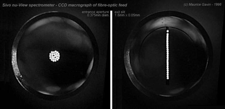
A fibre optic link connects the telescope to the spectrometer. At the telescope end, the fibre attaches to a brass coupler, which fits into the eyepiece tube. The link consists of a bundle of 25 fibre optic cables, each of 0.05mm diameter, that are arranged in an approximately circular pattern at the telescope end and are lined up to form a slit at the spectrometer end of the cable. Figure 2.4 shows both arrangements.6
This configuration results in spectral lines appearing as a series of vertical slits across the CCD. It is useful to quantify the width of a spectral line on the CCD, w', given the width of the slit, w, using the equation7
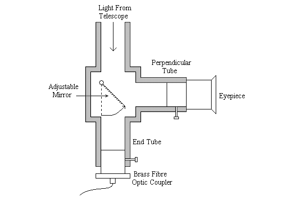
The observatory can be used for both imaging and spectroscopy. When imaging, the CCD is attached directly to the telescope and when being used for spectroscopy, the CCD is fixed to the spectrometer, which is in turn connected to the telescope via the fibre optic link. To make both applications practical, it is necessary to be able to alternate between viewing through an eyepiece and directing the light to the CCD/fibre optic bundle. This is made possible by the accessory shown in figure 2.5.
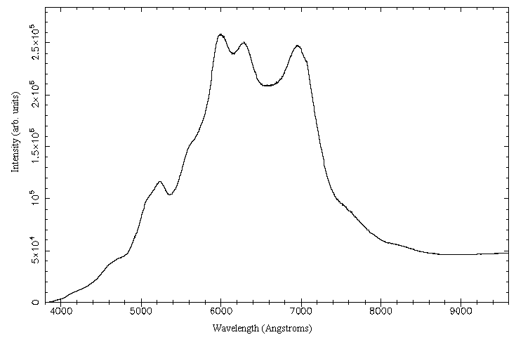
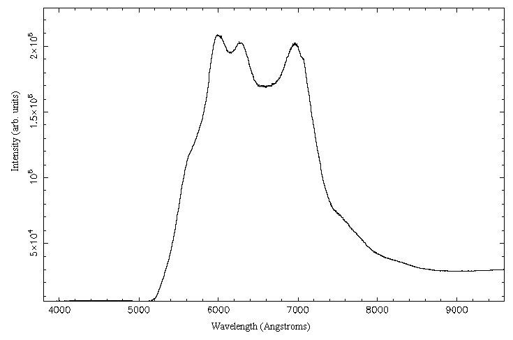
Due to the large wavelength range that can be covered and the nature of the grating, second order spectral lines can appear at long wavelengths. To prevent this a low wavelength filter is used. The CCD is sensitive up to wavelengths of approximately 10000Å, therefore a filter with a cut of around 5000Å is required. The effect of the filter can be seen by comparing the spectra of a tungsten bulb, taken with and without it, as shown in figures 2.6 and 2.7.
2.2 Experimental Method
2.2.1 Making Observations
The simplest kind of observation that can be made with the undergraduate observatory is the imaging of an astronomical object. Before this can be done, the CCD chip must be positioned in the focal plane of the telescope. To do this, a star was imaged with the CCD inserted into the telescope in a reproducible way. Repeated images were taken, refocusing the telescope each time, until the star appeared point-like in the image. For practical purposes, the CCD and eyepiece must be in mutual focus so that when refocusing is necessary, it can be done by eye instead of using multiple images. Therefore, once the CCD image was focused, the eyepiece was adjusted until it was also in focus.
In order to take an image of an object it must first be identified in the sky using a sky atlas or, in the case of planets, recent astronomical publications. Then it must be positioned in the field of view of the finderscope by moving the telescope to within a few degrees of the object. The telescope is adjusted to move the object to the centre of the finderscope and can then be fine-tuned to the centre of the eyepiece. An image can be taken of any exposure time between 0.01 and 3600 seconds.
Images can be adversely affected by both pixel noise and observing conditions. In order to account for this, a blank area of the sky can be imaged for the same exposure time as an image and later subtracted. This is called a dark frame. This technique proved particularly effective, as the same pixels stayed excessively warm and therefore noisy on a given night.
Spectroscopy is one of the most useful tools available to an astronomer. It allows the observer to extract astrophysical information such as the constituents of nebulae and stellar or planetary atmospheres. Another important application is the measurement of velocities through Doppler shifts.
Both the input and the output of the n -View need to be set up before the system can be used. The slit at the input must be aligned so that it is effectively parallel to the grooves in the reflection grating. The CCD at the output must be aligned so that the y co-ordinate of the chip is parallel with the slit image and inserted to the point where the chip is in the focal plane of the focusing lens. The first two stages are done by trial and improvement using multiple images. The last stage is done using a measuring dial attached to the top of the spectrometer, the value of which is known at the focus.
The fibre optic bundle is a very small target, so the telescope needs to be pointed very accurately in order for the light from an astronomical source to be incident upon it. This accuracy can be achieved by firstly inserting the 26mm eyepiece into the end tube with the more powerful 9mm eyepiece in the perpendicular tube. The source is then positioned in the central cross hairs of the weaker eyepiece. The graticule on the 9mm eyepiece is then used to ensure that the object is simultaneously in the centre of both. The brass coupler is then placed in the end tube providing a link between the telescope and spectrometer.
There is an approximately linear relationship between micrometer reading and centre wavelength of the spectral range illuminating the CCD. It was found that micrometer values of 3mm to 13mm in steps of 2 mm could be used to cover the practical spectral range of the CCD. Figure 2.8 shows the approximate spectral range of each micrometer setting used.
|
|
|
|
|
|
|
|
|
|
|
|
|
|
|
|
|
|
|
|
|
|
|
|
|
|
|
|
All spectroscopic data needs to be accompanied by spectra of calibration or arc lamps. The lamps contain elements with bright emission lines at well known frequencies and can be used to precisely calibrate the wavelength scale of the spectra. In order to use an arc lamp spectrum to calibrate an astronomical spectrum, the two must be taken at precisely the same micrometer setting and therefore wavelength range. The precision has to be such that the accuracy is greater than the limiting spectral resolution of the CCD. This can be crudely estimated using the fact that approximately 1000Å correspond to 375 pixels, giving approximately 3Å per pixel. The Vernier scale on the micrometer allows an accuracy of 0.001mm. Figure 2.8 indicates that there are approximately 500Å per mm and so the spectrometer is accurate to 0.5Å. Therefore, a single arc lamp spectrum can be used for each micrometer setting.
As with imaging, integration times of between 0.01 and 3600 seconds can be used to obtain spectra at any micrometer setting and therefore across the entire spectral range of the CCD. A dark frame of a blank part of the sky is also required to accompany each spectrum for analysis purposes.
In both imaging and spectroscopy, CCD images are downloaded to the standalone PC, where they can be saved into "fits" format for analysis.
2.2.2 Data Reduction
The non-spectroscopic images required no analysis as they were taken merely to investigate the application of imaging using the telescope/CCD system.
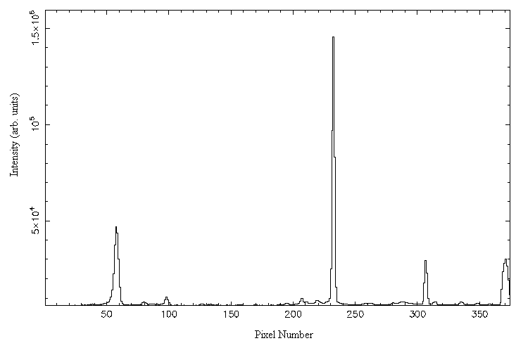
However, a number of reduction procedures are required to extract useful information from raw spectroscopic data. Firstly, raw spectra need to be cleaned. This involves subtracting the appropriate dark frame and removing the effects of cosmic rays that may have saturated certain pixels of the CCD. Then, the wavelength scale must be calibrated using an arc lamp spectrum at the appropriate micrometer setting. To do this, the emission lines in the arc lamp spectra need to be identified. A combination of helium and mercury arc lamps were used and the lines were identified using the ranges in figure 2.8 as a guide along with tables of emission line wavelengths and relative intensities.8 Raw arc lamp spectra, such as that shown in figure 2.9, can be loaded into a calibration program for this purpose.
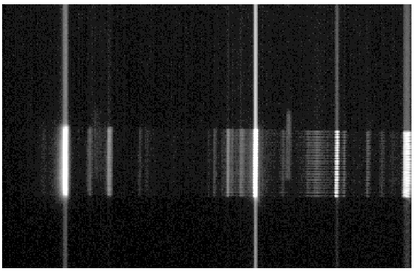
Figure 2.9. An example of a raw arc lamp spectrum. The brighter lines extend past the length of the slit. This is known as blooming and it does not effect the result as the intensity is integrated over the slit length only.
The program is given the range of y pixel values over which the data appears. It then integrates the spectrum over these values to produce a plot of intensity against x pixel value. An example of this, corresponding to figure 2.9 is shown in figure 2.10.
The lines that have been identified can now be selected and the appropriate wavelengths given to the program. The program then fits a dispersion relationship between wavelength and pixel number, which is exported to file so that the calibration can be applied to all spectra of the same micrometer setting. Appendix A contains the arc spectra used in calibration at each micrometer setting.
Once the calibration has been applied to the raw astronomical spectra, it is possible to integrate across the slit length to produce a plot of intensity against wavelength.
Starlink software was used to carry out the data reduction procedures.
2.3 Observations
2.3.1 images
Both Jupiter and Saturn were very conspicuous in the early evening sky for the duration of this project and so made easy targets for imagery. Several images of Jupiter and its moons were taken, an example of which is shown in figures 2.11 and 2.12. The moons are not nearly as bright as Jupiter, so the image must be slightly over-exposed for them to be seen more easily.
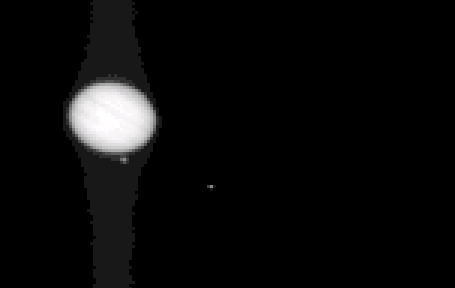
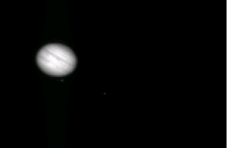
The bands of cloud in the upper atmosphere of Jupiter are clearly visible in figure 2.12.
Saturn was also imaged, an example is shown in figure 2.13.
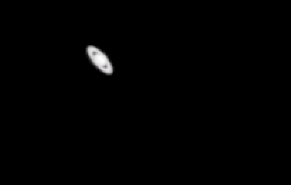
Although a ring is clearly visible, no structure can be resolved using the undergraduate observatory. The resolution required to detect the Cassini Division, which separates the two main rings, can be estimated using its width and the distance to Saturn. Saturn was approximately in opposition when this image was taken and orbits at a distance of 9.54 AU from the Sun,9 meaning that it was approximately 8.54 AU from Earth. Using the small angle approximation and the width of the Cassini Division to be 4800 km,9 the angle subtended was 0.77 arcsec. This is theoretically resolvable with the telescope but atmospheric seeing, along with the finite pixel size of the CCD prevent it.
2.3.2 Daytime Sky
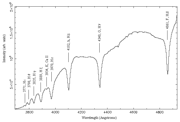
The easiest astronomical spectrum to obtain is that of the daytime sky. The light from the sky is sunlight that has been scattered in the ionosphere and undergone absorption due to molecules present in the Earths atmosphere. Therefore, a daytime spectrum is effectively a spectrum of our Sun with additional absorption. The main feature of interest in the solar spectrum is the Fraunhofer lines. These lines arise due to absorption by atoms and ions such as hydrogen and calcium in the solar atmosphere. Figure 2.14 shows the blue end of the solar spectrum.
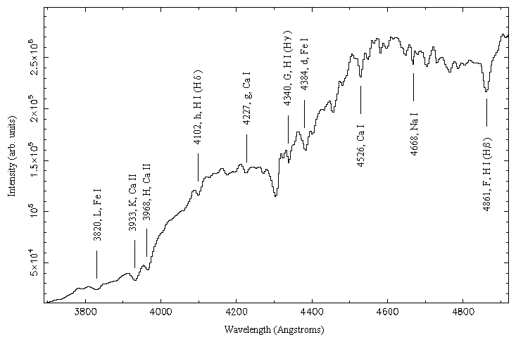
Figure 2.14. Spectrum of the daytime sky at low wavelengths with some of the strongest Fraunhofer lines indicated. Labels are of the form: wavelength, Fraunhofer designation (where available), element responsible for absorption.10
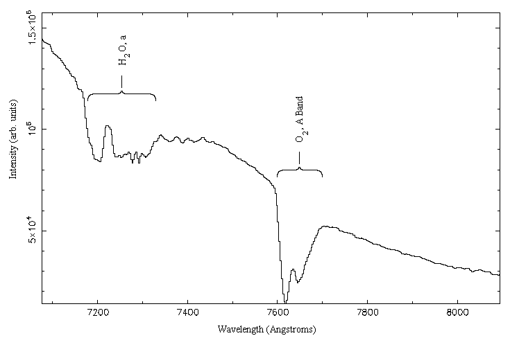
Molecular atmospheric absorption begins to become apparent towards the infrared end of the spectrum. This can clearly be seen in figure 2.15.
2.3.3 Jupiter
The combination of Jupiters appreciable angular size and its ideal position in the sky made it the simplest nighttime source for spectroscopy. As the light from Jupiter is reflected sunlight, its spectrum is very similar to that of the daytime sky. However, there are additional absorption features due to the presence of molecules in Jupiters atmosphere, most notably methane. A number of methane absorption features were observed when the Jupiter spectra were compared with those of the daytime sky. These are shown in figures 2.16 to 2.18.
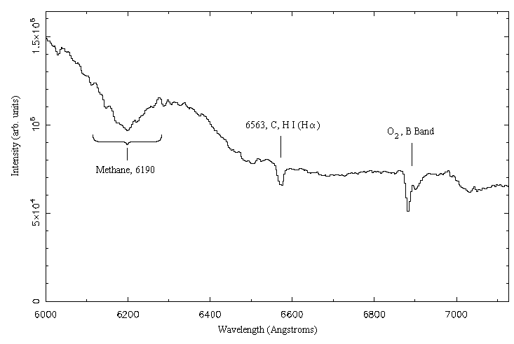
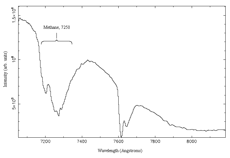
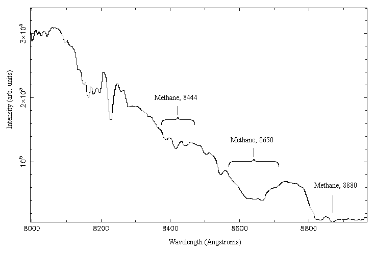
It has been known since 193214 that Jupiters atmosphere contains Methane. However, it is pleasing to be able to detect and identify it using the undergraduate observatory.
2.3.4 Vega
One of the most spectroscopically interesting stars is the bright A0 type star Vega. Stars of this spectral classification have a high abundance of hydrogen in their atmospheres, giving rise to a strong Balmer series dominating the blue end of their spectra. Calcium absorption lines are also expected, although not so much in Vegas end of the class.
Obtaining the spectrum of a star is more challenging due to the point-like appearance. Even if the graticule is set extremely accurately, the light may not pass down every fibre of the bundle in the fibre optic link. The effect of this is obvious in figure 2.19.
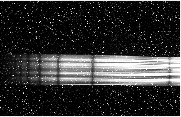
Figure 2.20 shows the same region of Vegas spectrum after analysis. Comparison clearly shows that there is more information in the raw spectrum than is initially apparent.
The wavelengths of the Balmer series, l n, are calculated from quantum theory, using the equation
The dominant Balmer series, evident in the spectrum of Vega taken with the undergraduate observatory serves as an elegant demonstration of undergraduate quantum mechanics of the hydrogen atom.