Supplementary Material to:

An Introduction to Radio Astronomy

4^th edition Cambridge University Press 2019

Last updated 28/06/2019

Chapter 9: The Basics of Interferometry

An E-W adding interferometer observing the Sun – a practical example

Section 9.1.2 gives a basic introduction to adding interferometry based on the analysis of a fixed East-West baseline and monochromatic (single frequency) operation; Fig 9.3 shows the idealised linear response of a single 20λ baseline to a perfect point source, which dominates the receiver noise, moving across the meridian and through the fringe pattern. The envelope of the fringe pattern is set by the beam of the primary antennas whose dimension is 2.4λ.

In the diagram above:

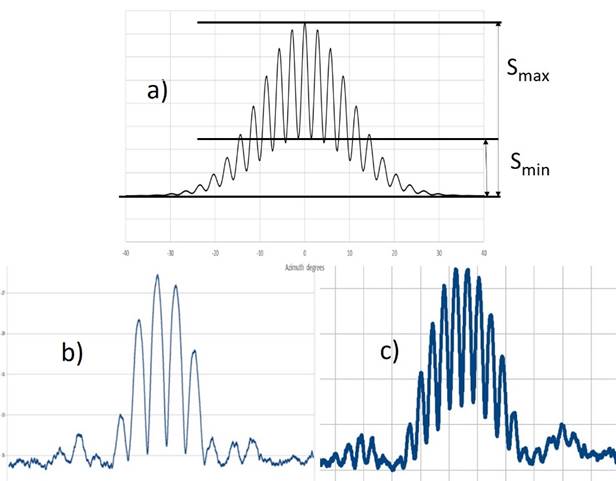
Pattern a) is the response of the same simulated baseline as in Fig 9.3 but now to a source whose size is comparable to the fringe spacing; the effect of resolution is clear. Following the original definition of fringe visibility by Michelson and the analysis in Chapter 6 of the classic text book “Radio Astronomy” by J.D. Kraus the visibility V on a particular baseline is:

V = [S_max - S_min]/[S_max + S_min]

where S_max and S_min are measured in linear units above a defined “off-source” level.

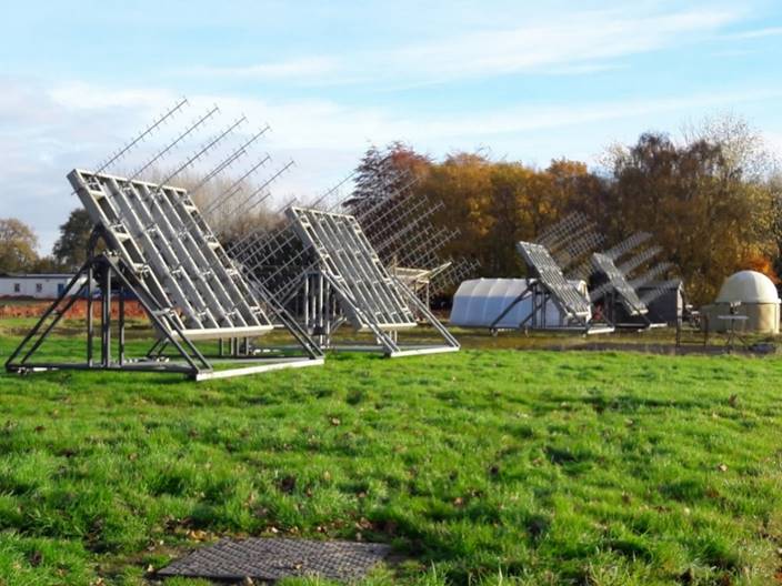
The real-life plots in b) and c) above are actual observations taken with one baseline (i.e. between two frames) of the 4-frame MUST interferometer at Jodrell Bank Observatory (image below); Fig 8.12 in the main text shows a close-up of one of the frames.

The source was the Sun, the frequency was ~600 MHz and the fractional bandwidth of the receiving system was 5 MHz (i.e. <1%) thus the interferometer was essentially operating in monochromatic mode. The received power from the two frames added together is plotted on a logarithmic scale with respect to the system noise power (i.e. the “off source” level).

Pattern b) was taken with a short baseline (20 λ thus fringe spacing = 2^o.9) and so the disk of the Sun (diameter 0^o.5—0^o.6 at this frequency) is barely resolved (V ~ 0.95).

Pattern c) was taken with a ~2x longer baseline, note the reduced fringe separation; the disk of the Sun is now clearly resolved (V ~0.8). By plotting V as a function of baseline the angular diameter of the Sun’s disk can be measured – see the discussion in Section 9.4.3 and Fig 9.15 (and below) .

Note also the additional fringes outside the main pattern, they reveal the first sidelobes of the square frame arrays seen in Fig 8.12. (Credit: E. Vavilina; G. Gaigals; P. Wilkinson)

Adding interferometers: constructing visibility amplitudes for point and gaussian double sources

In simple cases (as above and Section 9.4.3) it is possible to infer the structure of the source from the variations in visibility amplitude alone. The case of double sources is treated in the schematics below:

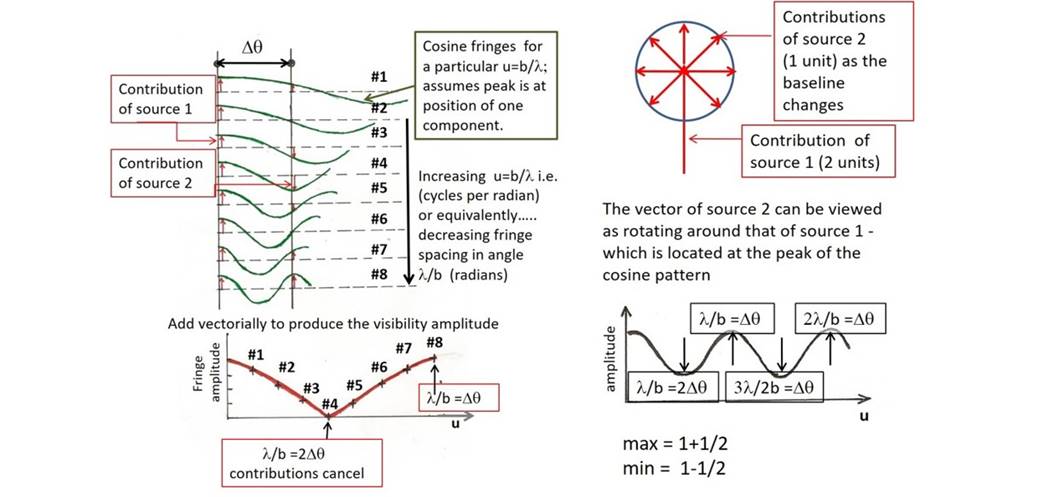
Top left: an equal double point source, separation Dθ (radians) is observed with baselines (b) of increasing length (#1 to #8); the corresponding fringes are plotted in green. The two sources fall on different parts of each cosine fringe and their contributions add vectorially.

Bottom left: the resultant visibility plotted in terms of the number of wavelengths in the baseline (u=b/λ). The cosine Fourier transform of two points appears and when the fringe spacing 1/u= λ/b=2Dθ the contributions of the two components cancel out and the visibility amplitude reaches a zero null.

Top right: If the two point sources do not have equal flux densities then the modulation of the visibility function is reduced. The maximum is the sum of the fluxes and the minimum is the difference.

Bottom right: the resultant visibility vs. baseline plot. The range of baseline lengths plotted is longer than in the left hand plot. .

If the two components have a similar shape (e.g. a circular gaussian) the source structure is described by the convolution of a point double with that shape. From the Convolution Theorem the visibility amplitude is that of the point double multiplied by the Fourier Transform of the component shape (see Figure 9.17 in the main text and below).

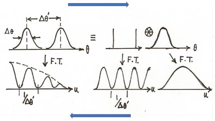
Top line: A double gaussian source is obtained by convolving two point sources with a single gaussian

Bottom line: the Fourier Transform the components together with the convolution theorem; the FT of the gaussian double is obtained by multiplying the component transforms.

The value of model fitting to interferometer data

Correlation interferometry is introduced in section 9.1.3 and in general leads on to the full panoply of aperture synthesis imaging described in Chapters 10 and 11. However, model fitting to the data in the visibility (u,v) plane still has a useful research-level role to play in certain niche circumstances. Pearson (1999) provides clear introduction to the philosophy and the techniques; a recent practical software suite UVMULTIFIT is described by Marti-Vidal et al (2014).

A typical application is when the source is known/thought to be relatively simple a priori but the visibility data are sparse and so the standard synthesis imaging approach of self-cal + deconvolution may be operating at, or perhaps beyond, the limit of its reliability. Modelling of the available visibilities then provides a practical means of obtaining a quantitative description of the source. By assuming an analytic shape for components in the source one is implicitly supplying additional a priori information (including sky positivity) to aid the interpretation of the brightness distribution. Current applications include intercontinental VLBI observations at mm wavelengths and space VLBI. A recent example of modelling of mm-wave VLBI data on Sagr A* in the Galactic Centre is given by Issaoun et al (2019) https://arxiv.org/abs/1901.06226 . Paper VI in the series describing in detail the observations and data analysis of the M87 black hole shadow by the Event Horizon Telescope consortium (2019) https://arxiv.org/abs/1906.11243 highlights the continued astrophysical importance of model fitting directly to the visibility data; in this case the closure phases and closure amplitudes (see section 10.10) were also used as constraints.

Visibility modelling is also useful for making quantitative estimates of the brightness temperatures of compact sources (Chapter 16; Lobanov 2015). Modelling can also be useful when the basic structure of an evolving source is known and successive models made at different epochs enable the evolution to be followed quantitatively; examples are the expansion of the shell of a young supernova remnant or the motion of a knots in the jet of a superluminal source (AGN or X-ray binary).

An early example – I: the radio jet in the giant elliptical galaxy M87

In the early 1970s aperture synthesis arrays had not achieved sub-arcsecond resolution but pioneering phase-stable observations were being made on radio-linked baselines using telescopes at Jodrell Bank and extending to ~25m paraboloids ~24km (MkIII telescope) and ~126 km (Defford telescope) away. As described by Wilkinson (1974) success was achieved using data from these interferometers to elucidate the radio structure of the M87 jet for the first time (see Fig 16.8 for the later VLA images).

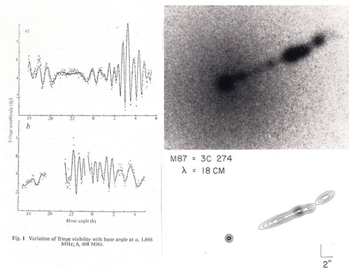
Top left panel: Single baseline fringe amplitudes at 1666 MHz (λ=18cm) to the MkIII telescope (baseline 132,300 λ ) and 408 MHz ((λ=74cm) to the Defford telescope (baseline 172,700 λ) with the solid lines being the visibilities calculated from the gaussian models listed in the bottom panel.

Top right panel: A contemporaneous optical image of M87 showing the jet (compare with the modern optical image in Fig 16.8). Below it is a contour representation of the multicomponent gaussian model made from the λ=18cm data obtained with the Jodrell Bank – MkIII baseline.

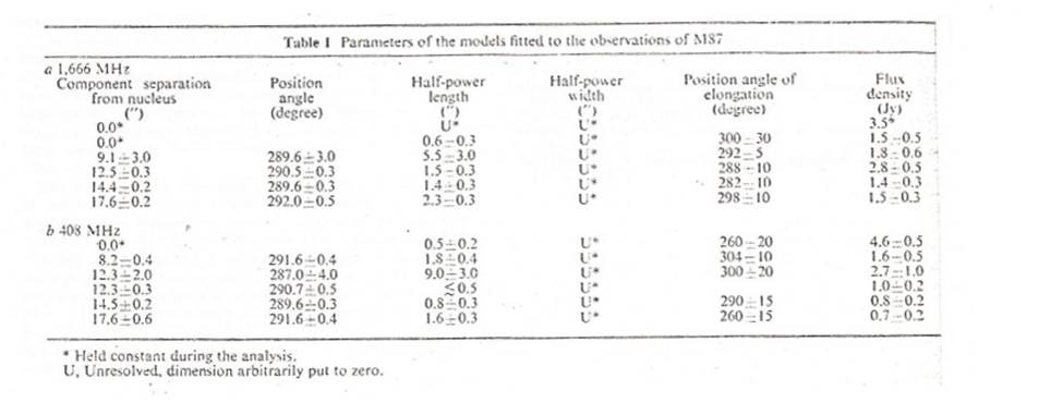
Bottom panel: The gaussian model components fitted to the visibility data from the Jodrell Bank – MkIII baseline (1666 MHz; λ=18cm) and the Jodrell Bank – Defford baseline (408 MHz λ =74cm).

When carrying out these model fits the author did not know the detailed optical structure of the M87 jet shown in the image to the top right but the complexity of the interferometric visibility variations required multi-component models in order to follow them. As described by Wilkinson (1974) these models showed for the first time that that the structure of the M87 jet is essentially the same over a frequency range of ~10⁶:1.

Reference: Wilkinson, P.N. 1974 “Radio structure of the M87 jet”, Nature, 252, 661

An early example – II: the radio jet in the quasar 3C147

In the mid-1970s the first VLBI image that could justifiably be termed an aperture synthesis image was made (Wilkinson et al 1976). The CLEAN + closure phase technique outlined in Section 10.10 was used to map the core plus radio jet in the bright quasar 3C147. The technique, the convergence process and the assessment of its reliability with “blind” testing is described by Readhead & Wilkinson (1977). While focussing on the new mapping technique the paper on 3C147 also demonstrated the power of model fitting to visibility data.

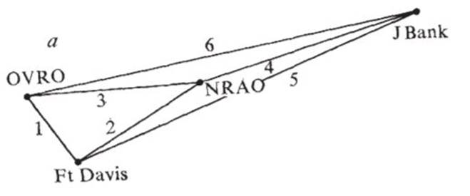
The VLBI data were taken in two independent observing runs both centred at 609 MHz ( λ50cm) . The first run in 1973 involved three US telescopes at Owens Valley, California (OVRO); Ft. Davis, Texas and Green Bank, West Virginia (NRAO). The second run in 1975 added the transatlantic baseline to Jodrell Bank (UK). The disposition of the baselines in the 1975 observations is shown schematically below

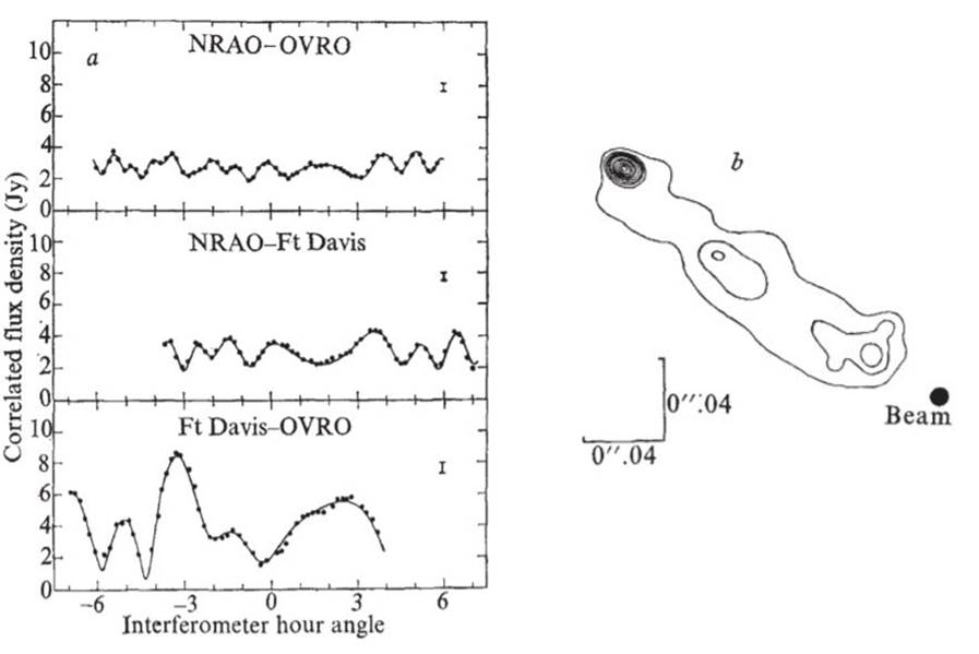
The 1973 US-only data were analysed by G.H. Purcell by model-fitting to the visibility amplitude data since at this time the closure phase mapping technique had not been developed. The high quality visibility amplitudes and a contour representation of the inferred brightness distribution from Purcell’s 13-gaussian model are shown below. The original gaussian components were convolved with a circular gaussian (FWHM = 0”.009) to simulate the effect of the CLEAN beam in the 1975 map shown below.

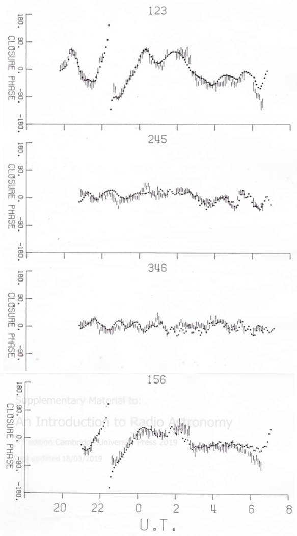
The power of visibility amplitude model-fitting is demonstrated by the set of closure phases from the 1975 data shown in the diagram below; the dotted lines are the calculated closure phases from on Purcell’s model using the visibility amplitudes from the three US-only baselines. The baseline numbering is given in the diagram above and note that only three closure phases are independent. The close similarity between the 1973-based model fit and the independent 1975 closure phases is striking and provides another demonstration of the utility of visibility model-fitting.

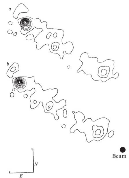
The “hybrid map” of 3C147 which made full use of the closure phases is shown below; the two versions are the results of different starting models (see Wilkinson et al 1974 for more details). Note that these maps made no positivity or smoothness assumption (both implicit in gaussian model fitting) and also unambiguously set the SE-pointing direction of the jet; the gaussian model could be rotated through 180^o and still produce the same visibility amplitudes. Nowadays the closure phases (see Chapter 10 and Pearson 1999) would be used to provide further strong visibility constraints on the model-fit.

Both the above cases from the 1970s served to demonstrate that useful astrophysical inferences can be made using visibility amplitude modelling alone.

References

Wilkinson, P.N., Readhead, A.C.S., Purcell, G.H. and Anderson, B. 1977 “Radio structure of 3C147 determined by multi-element very long baseline interferometry”, Nature, 269, 764.

Readhead, A.C.S. and Wilkinson, P,N. 1978 “The mapping of compact radio sources from VLBI data”, ApJ, 223, 25

The 1-D visibility amplitudes of some simple sources

As a start to the modelling process it is often useful to look at 1-D cuts through the visibility functions of simple sources; Pearson (1999) and Thompson Moran and Swenson (Section 10.4) discuss some examples. To complement these discussions and the main text section 9.4.3 we have calculated visibility amplitudes for the following circularly symmetric sources with the characterising angular dimensions given in brackets:

· a gaussian (full width half maximum)

· an annulus (inner radius = 0.8x mean; outer radius = 1.2 x mean radius as illustrated below)

· a uniform disk (radius)

· an infinitely thin ring (radius)

To these we have added:

· an equal point double (separation)

Pearson (1999) and Thompson Moran and Swenson (Section 10.4) provide analytic formulae. For completeness we also give them here, adding the case of a point double. The reader should note the difference in the formulae quoted in terms of diameter (Pearson 1999) and radius (TMS); we have used the latter.

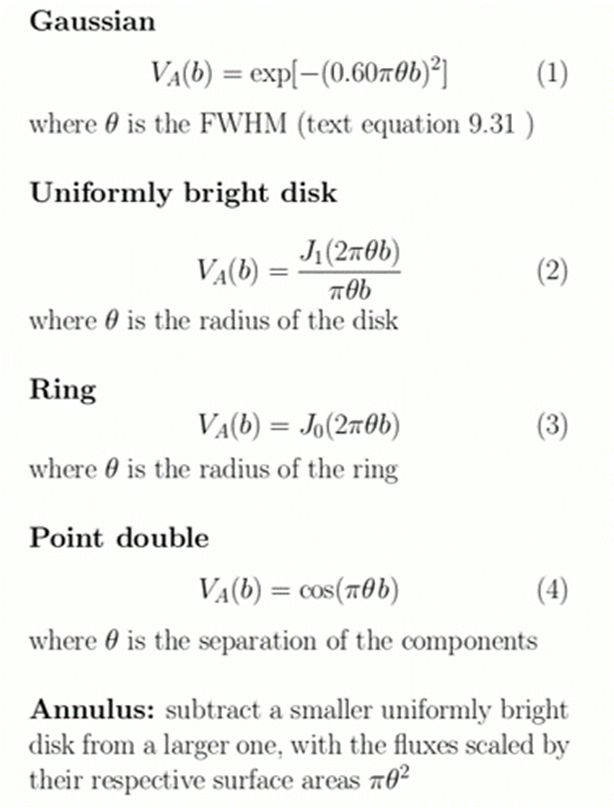
Formulae for the normalised visibility amplitudes V_A for a baseline b (wavelengths)

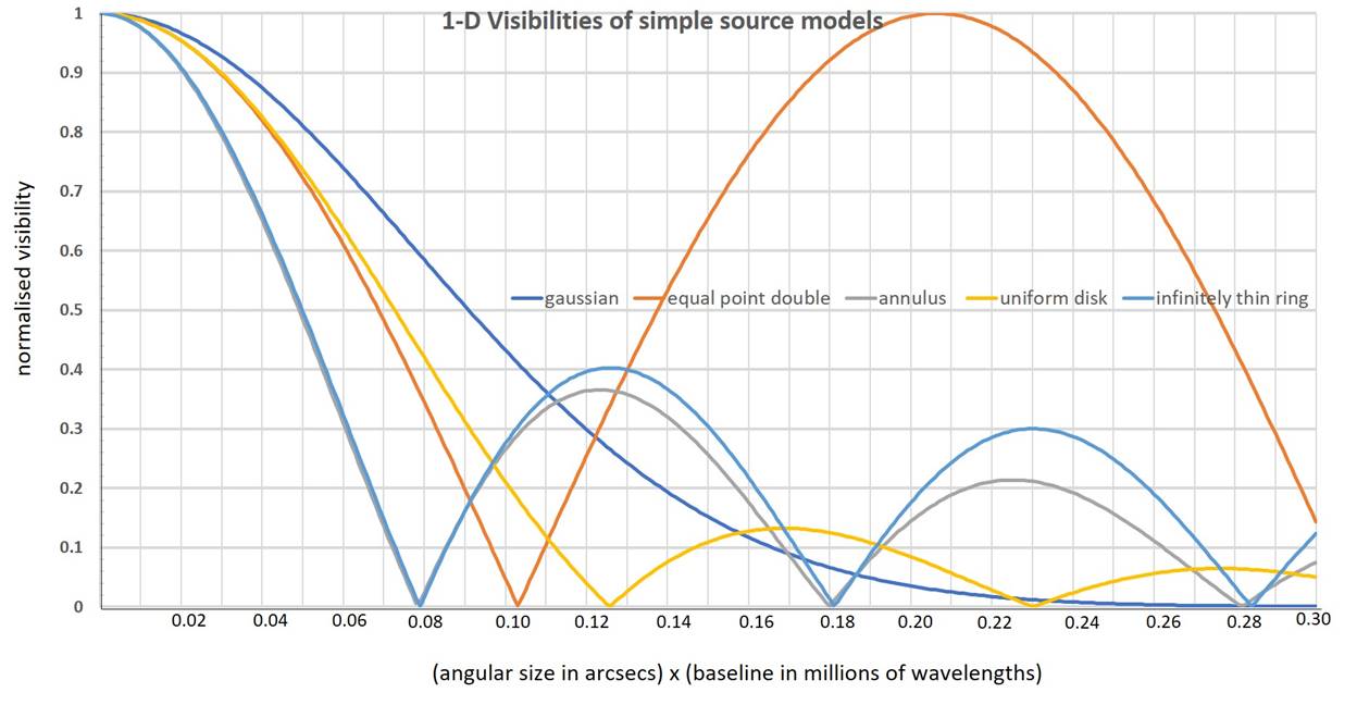
Plots of the normalised visibility amplitudes

Note that these are visibility amplitudes from a correlation interferometer with only the magnitude of the Fourier Transform shown. For sources exhibiting visibility minima the phase reverses at each successive minimum. For example an equal double source has a cosine transform (as opposed to the [1+cosine] form for an adding system - see above and section 9.4.3) but the negative going part of the cosine is reflected about the horizontal axis when only the amplitude is required.

Looking at this 1-D visibility function plot several qualitative points emerge

1. A gaussian source never shows a visibility minimum – this is because the brightness distribution has no “sharp edges”

2. The visibility of equal point double can easily be transformed into that of a double with resolved gaussian components by multiplication (see diagrams above)

3. The visibility of an infinitely narrow ring and a finite width annulus are similar until after the 2^nd minimum – stressing the need for long baselines to distinguish between them.

4. The visibilities of the thin ring and annulus are noticeably different from that of the uniform disk.

To interpret this plot quantitatively select a normalised visibility value and then look to the ordinate for the product of characteristic angular size= θ (arcsec) and 1-D baseline = B (Mλ). For example for a measured visibility = 0.5

· gaussian θ.b= 0.092

o θ (FWHM) = 0.092 arcsec for a 1 Mλ baseline; θ (FWHM) = 0.00092 arcsec for a 100 Mλ baseline

· annulus θ.b= 0.078

o θ (mean radius) = 0.078 arcsec for a 1 Mλ baseline; θ (mean radius) = 0.00078 arcsec for a 100 Mλ baseline

· uniform disk (radius) θ.b= 0.126

o θ (radius) = 0.126 arcsec for a 1 Mλ baseline; θ (radius) = 0.00126 arcsec for a 100 Mλ baseline

· thin ring θ.b= 0.078

o θ (radius) = 0.078 arcsec for a 1 Mλ baseline; θ (radius) = 0.00078 arcsec for a 100 Mλ baseline

· equal point double (separation) θ.b= 0.069

o θ (separation)= 0.069 arcsec for a 1 Mλ baseline; θ (separation) = 0.00069 arcsec for a 100 Mλ baseline

Alternatively focus on the position of the 1^st minimum:

· gaussian – no minimum

· annulus θ.b= 0.078

o θ (mean radius) = 0.078 arcsec for a 1 Mλ baseline; θ (mean radius) = 0.00078 arcsec for a 100 Mλ baseline

· uniform disk (radius) θ.b= 0.073

o θ (radius) = 0.073 arcsec for a 1 Mλ baseline; (radius) = 0.00073 arcsec for a 100 Mλ baseline

· thin ring θ.b= 0.078

o θ (radius) = 0.078 arcsec for a 1 Mλ baseline; (radius) = 0.00078 arcsec for a 100 Mλ baseline

· equal point double (separation) θ.b= 0.103

o θ (separation)= 0.103 arcsec for a 1 Mλ baseline; θ (separation) = 0.00103 arcsec for a 100 Mλ baseline

Another instructive way of looking at these visibility functions is to scale the characteristic sizes of the sources so that their visibilities fall to 0.5 at the same baseline (see Pearson 1999). The size scalings with respect to the plot above are:

· gaussian (full width half maximum) x 1.82

· annulus (mean radius) x 1.00

· uniform disk (radius) x 1.45

· infinitely thin ring (radius) x 1.00

· equal point double (separation) x 1.38

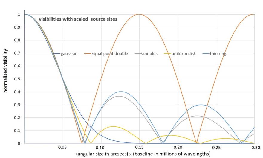
It is clear that, unless the normalised visibility function is traced, with good signal-to-noise ratio, below ~0.2 and beyond the first minimum, these quite different brightness distributions will not be readily distinguished from the visibility data. The characteristic dimension assigned to the source, and hence its brightness temperature, will therefore be subject to significant uncertainty.

The May 2019 Center for Astrophysics colloquium on the M87 black hole shadow by Shep Doeleman (P.I. of the Event Horizon Telescope consortium) illustrates the value of familiarity with the visibility functions of simple models such as those above see https://www.youtube.com/watch?v=oFF0ES-OhfY (between 21:25 and 22:30 after the start).

References

Event Horizon Consortium (2019) https://arxiv.org/abs/1906.11243

Lobanov, A., “Brightness Temperature Constraints from Interferometric Visibilities”, Astron. Astrophys., 574, A84 (9pp) (2015)

Martí-Vidal, I., Vlemmings, W.H.T., Mueller, S., and Casey, S., “UVMULTIFIT: A Versatile Tool for Fitting Astronomical Radio Interferometric Data”, Astron. Astrophys., 563, A136 (9pp) (2014)

Pearson, T.J., “Non-Imaging Data Analysis”, in Synthesis Imaging in Radio Astronomy II, Taylor, G.B., Carilli, C.L., and Perley, R.A., Eds., Astron. Soc. Pacific Conf. Ser., 180, 335–355 (1999)

Wilkinson, P.N. “Radio structure of the M87 jet” Nature, 252, 661 (1974)