Supplementary Material to:

An Introduction to Radio Astronomy

4^th edition Cambridge University Press 2019

Last updated 04/12/2021

Chapter 8: Single-aperture Radio Telescopes

A corrugated horn feed:

The commonest feed design used in radio astronomy systems (section 8.1) employs surface corrugations between λ/4 and λ/2 in depth. The modified surface avoids a discontinuity at the edges of the horn aperture. The flexibility allowed by such an arrangement allows broad band reception coupled with good control of the beam pattern and polarization purity.

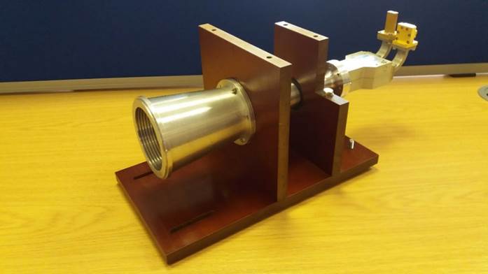
A corrugated horn feed for K-band (centre frequency 22 GHz) mounted in a test fixture and with a circular polariser on the output. The horn has an internal diameter of 65mm at the open end. (courtesy E. Blackhurst)

Phased Array Feeds (PAFs): ASKAP and APERTIF

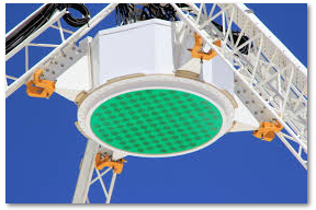
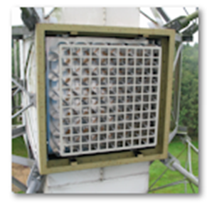
PAFs are revolutionising the field-of-view available to dishes. The ASKAP PAF (left) is a close-packed planar array of 94 dual-polarization dipoles – see https://www.csiro.au/en/Research/Astronomy/ASKAP-and-the-Square-Kilometre-Array/PAFs which covers the range 700-1800 MHz with an instantaneous bandwidth of 300 MHz available. The APERTIF feed (right), developed at ASTRON in the Netherlands uses a box-like structure of close-packed Vivaldi tapered slot dipoles (see www.apertif.nl ).

Both feed systems are designed for L-band operation and can produce up to 30 close-packed beams on the sky hence greatly extending the field-of-view (FoV) of the telescope. Careful adjustments of the complex weights applied to the elements forming each beam (see main text Fig 8.27) can also improve the aperture efficiency over that of a “standard” feed and hence increase the telescope’s effective area A_eff. The great advantage of PAFs is the increase in the survey speed which, for a given bandwidth, is proportional to FoV x [Aeff/T_sys]² (see the new section at the end of Supp. Mat Chapter 11). However, both these L-band PAFs are uncooled for reasons of cost and complexity and the achieved T_sys values are typically a factor two higher than for a cryogenically-cooled single feed receiver, this partly offsets the FoV and A_eff improvements. Several groups around the world are, therefore, now developing cryogenically cooled PAFs.

Measured antenna power patterns

Fig 8.15 shows a highly idealised power pattern of an antenna in polar coordinates. Below we show three actual plots of antenna power patterns taken from student experimental work at the Jodrell Bank Observatory.

Low-cost “cantenna” feed

A low-cost “cantenna” (an open circular waveguide) for feeding a small (3.1m) parabolic dish at 21cm wavelength was constructed out of a food can (top left) with a type-N connector and λ/4 probe (drawing bottom left). The beam pattern plotted in Cartesian coordinates is shown at the top right and in polar coordinates at the bottom right. The data were taken at 5^o intervals and normalised to 0 dB on axis, the FWHM is ~65^o and the peak backlobe is -15 dB (credit Abeer Almutairi). Many websites provide detailed information on the design and construction of cantennas.

Commercial Yagi

This commercial 16-element Yagi antenna was designed for UHF broadcast TV reception in a band near 600 MHz; a planar phased array of these antennas in the MUST facility is shown in Fig 8.12. Left) a schematic of the antenna configuration (credit E. Vavilina); right) a power pattern, plotted in polar coordinates, taken on a temporary outdoor range. The data were taken at 5^o intervals and normalised to 0 dB on axis, the FWHM is ~30^o and the peak backlobe is -19 dB.

Experimental Corrugated Horn

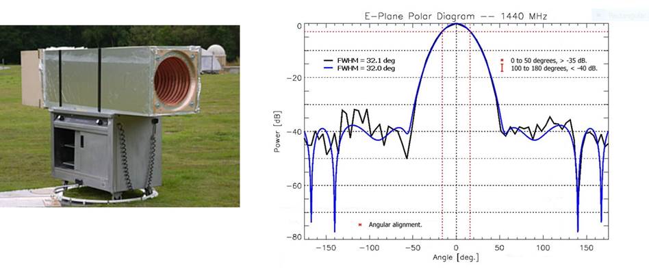
Left) An experimental low-cost corrugated horn antenna (aperture 0.55m) built to assess a novel construction technique and its potential for future radio astronomy projects at L-band. Right) the measured (black) and calculated (blue) power patterns plotted in Cartesian coordinates. The sidelobes are much lower than those of the Yagi antenna and the agreement with theory is good; note however that accurate measurements at the -40dB level in the field are subject to residual scattering despite the use of a large ground screen (not shown). (credit I.W.A.Browne & A. Colclough).

Feed illumination, surface profiles and power beam of a parabolic dish via holography

(Section 8.8 and Chapter 9)

The accurate surface profile of a dish can be determined in several ways: by laser scanning, by photogrammetry or, as here, using radio holography. In this technique a distant source, often a satellite transponder but a powerful celestial radio source can also be used, is observed with an interferometer. The dish under test (DUT) acts as one element and is raster scanned across the target source while the beam of the other element remains fixed on the source. By this means the complex voltage polar diagram of the DUT is obtained; the complex field across the aperture of the DUT can then be obtained by Fourier transformation. From the phase pattern the variations in surface profile in wavelengths (and hence mm) can be obtained.

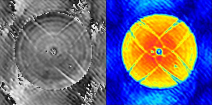
(Left) the phase and (right) the amplitude components of the complex illumination pattern of the Torun 32-m dish obtained during the late stages of a holographic programme using the Eutelsat w2 satellite transponder at 12.1 GHz. In both patterns the shadow of the secondary mirror support legs can be seen; a test panel, which has been mis-set from the overall parabolic shape, can also be seen in the lower right quadrant. The amplitude pattern shows the effect of the feed taper; less power is collected from the outer parts of the dish.

Left) the phase deviations have been translated into wavelengths and hence mm away from the desired parabolic profile. A calibration panel (height 3 mm) can be seen in the lower right hand quadrant. After the holographic resetting the overall surface rms was ~0.4mm rms corresponding to a reflectivity of ~78% at an observing frequency of 30 GHz (wavelength 10mm; Ruze formula). Prior to resetting (see profile patterns below) the surface rms was 0.8 mm rms corresponding to a reflectivity of 36% at 30 GHz. (right) the corresponding beam pattern, the larger sidelobes in p.a. ±45^o are due to blocking/scattering of radiation by the secondary mirror support legs.

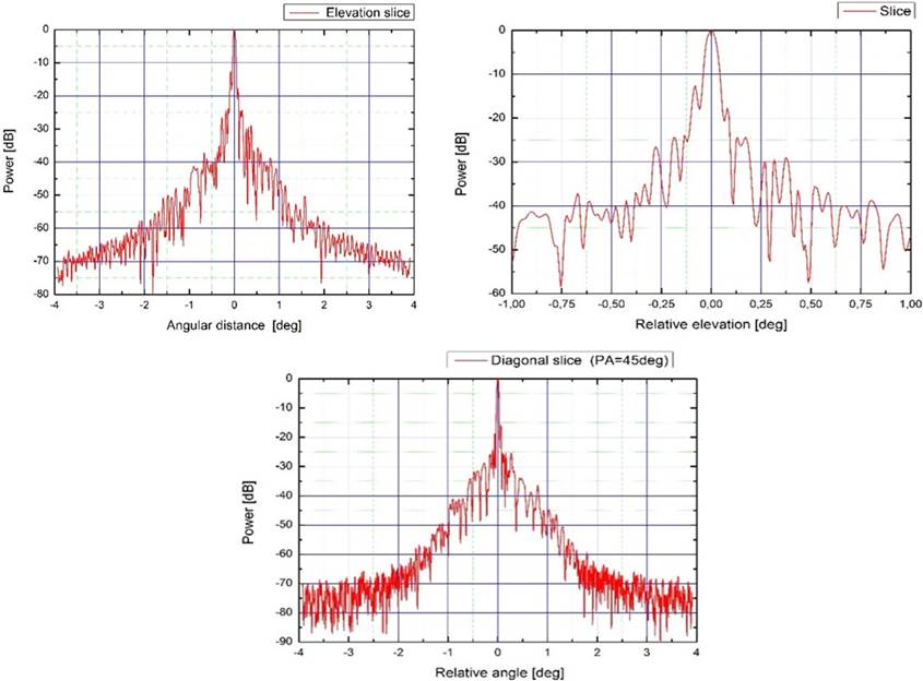
1-D cuts through the above beam pattern expressed in dB relative to the peak. The top panel shows a vertical cut (in elevation) over two angle ranges (±4^o and ±1^o). The bottom panel shows a cut at 45^o over a ±4^o range; the higher level of the sidelobes in this direction can clearly be seen.

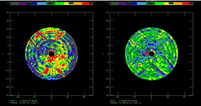
Left) The surface profile at an early stage in the holographic measurement programme when the setting accuracy was 0.8 mm rms; right) the surface profile after a first stage of resetting. Note that in this stage different test panels were set up compared to that used in the final resetting stage shown above.

IMAGE CREDIT: A Kus and G. Pazderski (TcFA Torun)

For recent detailed descriptions of the use of holography to characterise radio antenna beams see

· “Primary beam effects of radio astronomy antennas: I. Modelling the Karl G. Jansky Very Large Array (VLA) L-band beam using holography” by K. Iheanetu et al. (2019) https://arxiv.org/pdf/1903.02486.pdf

· “Primary beam effects of radio astronomy antennas: I. Modelling the MeerKAT L-band beam ” by K. Iheanetu et al. (2019) https://arxiv.org/pdf/1904.07155.pdf

Voltage and power beams – a pictorial recapitulation (Sections 8.3 and 8.9)

N.B. antenna size is denoted by D in the main text not d as in the diagram below

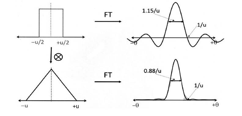
Left) There is a “Fourier pair” relationship between the spatial pattern of the electric field illumination across the aperture (the aperture distribution) and the angular pattern of the complex electric field in the far-field (the “voltage beam”): this is a basic result from Fraunhofer diffraction theory. Here, for simplicity, the illumination pattern is drawn as 1-D cut through a uniformly-illuminated square antenna and the voltage beam is therefore a sinc function. Note that at a given frequency the voltage beam oscillates from negative to positive at the radio frequency i.e. typically at GHz rates. The power beam, being the voltage beam squared, does not oscillate.

Right) The Wiener-Kinchin theorem states that the power spectrum of a function is the Fourier transform of its autocorrelation function (ACF). In this case the power spectrum is the angular spectrum of the power beam and the ACF is that of the antenna aperture distribution. The power beam is therefore a sinc² function. Note that although the ACF is has twice the extent of the uniform distribution its tapered shape gives a power beam which does not have double the formal resolution of the voltage beam in particular the 1^st zero in sinc² and sinc is at 1/u. The FWHM of the intensity main beam (left) is, however, narrower than that of the voltage beam (right) as shown in the main text Fig 8.20 and reproduced here.

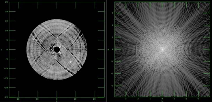
Beam smoothing and angular frequency cut-off

The “true” sky distribution (intensity or power) can be viewed as either

· a fine grid of point sources to be convolved with the (spatial) antenna power beam

or

· a spectrum of angular frequency components with units of cycles radian^-1 (compare with Hz i.e. cycles s^-1) to be weighted by the angular frequency “transfer function” of the antenna for intensity.

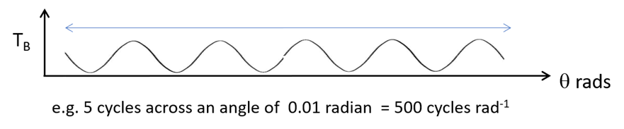
In the first case convolution with the antenna power beam smooths out fine details in the spatial temperature distribution of the sky on angular scales smaller than ~λ/D i.e. smaller than 1/u (Figs 8.31 and 8.32). In the second case we consider the sky temperature distribution (intensity or power) as made up of Fourier components of different angular frequencies (number of cycles rad^-1 across sky) e.g. 500 cycles rad^-1 in the figure below

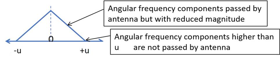
The antenna can be regarded as having a virtual “intensity aperture” (i.e. its angular frequency transfer function; the ACF of the aperture distribution) extending from -u to +u. For the specific case of a uniformly illuminated square aperture the ACF has a triangular shape but all distributions will fall away from the central peak. This transfer function implies an increasingly low weighting to the higher spatial frequency Fourier components in the sky brightness distribution; it acts as a low-pass filter cutting out angular frequencies greater than u: hence the smoothed sky distribution is “band-limited” i.e. “cut-off” beyond u cycles/radian

In summary

State-of-the-art radio telescopes:

The historical development of the design and construction of reflector antennas used for radio astronomy is extensively covered in the book by J,M. Baars and H.J. Kärcher ” Radio Telescope Reflectors” pub. Springer 2017. This is available on the web at https://link.springer.com/content/pdf/10.1007%2F978-3-319-65148-4.pdf

Fixed Reflectors.

The telescopes with the largest collecting area are the fixed reflectors FAST and Arecibo. Their beams are swung over large angles by moving the feed. This requires compensation for aberration. In FAST this is achieved by deforming the flexible surface; the Arecibo surface is spherical, and compensation is achieved in a secondary feed and reflector system.

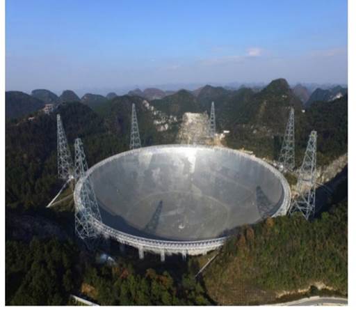
Five Hundred Metre Aperture Radio Telescope (FAST). Situated in Guizhou province in south-west China FAST is now the largest single dish in the world. The surface is active and can be pulled by over 2000 steel cables into a parabolic profile with a diameter of 300m. As the source moves across the sky the parabolic area and the suspended feed move under computer control to track it http://fast.bao.ac.cn/en/

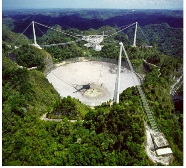
Arecibo Telescope. Situated in Puerto Rico and commissioned in the 1960s it was for over 50 years the world’s largest single aperture telescope with an effective diameter of ~200m. The reflecting surface has a fixed spherical profile and to correct for aberrations the focus area has secondary and tertiary mirrors

(www.naic.edu/ao/landing)

Dishes with adjustable surfaces.

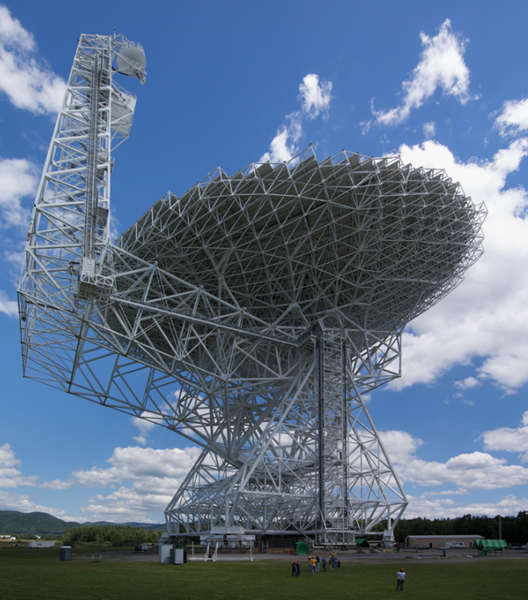
Green Bank Telescope (GBT). Currently the world’s largest fully steerable dish with a diameter exceeding 100m. The offset design was chosen to minimise scattering off the telescope structure and hence to reduce sidelobes (https://greenbankobservatory.org/telescopes/gbt. The surface panels are adjustable by over 2000 actuators under computer control. An overall surface accuracy of 240 μm rms. has been achieved which allows useful observations down to 3mm (110 GHz) wavelength to be made when the atmospheric opacity is low (for more details see Frayer et al (2018) https://arxiv.org/pdf/1811.00105.pdf ).

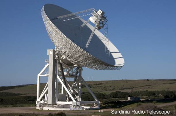
Sardinia Radio Telescope (SRT). The 64-m Sardinia Radio Telescope has an active surface controlled by over 1000 actuators; the specification of 150 μmr.m.s. enables operation to 3 mm wavelength with good efficiency. Designed for flexible operation for a variety of uses, including space communications, the SRT’s innovative optics permit a wide range of receivers to be operated at several focal stations (http://www.srt.inaf.it).

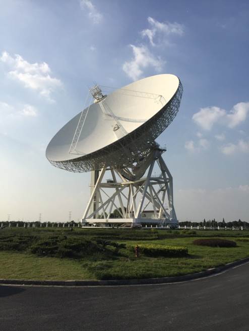
Tian Ma Telescope The 65-m Tian Ma telescope in Shanghai China was commissioned in part to support China’s Lunar Exploration project. It has Cassegrain optics and active surface control giving an overall accuracy of 300 μmr.m.s. allowing good performance up to 50 GHz (http://english.shao.cas.cn/fs/201410/t20141008_12893.html

Dishes at millimetre wavelengths

IRAM 30-m telescope at Pico Veleta (iram-institute.org) The Franco-German Institut de Radio AstronomieMillimetrique (IRAM) operates a 30-metre radio telescope, designed for millimeter-wave observations, on the Pico Veleta (altitude 285m) near Granada Spain. Its overall r.m.s. surface accuracy is 70 μm and is intended primarily for spectroscopic studies of the interstellar medium. To over- come the atmospheric emission from water vapor, it has a nodding secondary that allows comparison of the observing field with a reference field nearby (http://www.iram-institute.org/EN/30-meter-telescope.php)

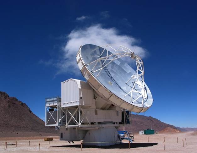
Atacama Pathfinder Experiment Telescope (APEX) The 12-m diameter APEX (Atacama Pathfinder Experiment)telescope is operated by a consortium of the Max Planck Institutf¨urRadioastronomie (MPIfR) at 50%, the Onsala Space Observatory (OSO) at 23%, and the European Southern Observatory (ESO) at 27%. It is situated on the Llano Chajnantor close to the ALMA array at an altitude of 5105m. The antenna is a modified ALMA prototype dish with an r.m.s. surface accuracy of 17 μm enabling it to operate at frequencies above 1000 GHz (http://www.apex-telescope.org).

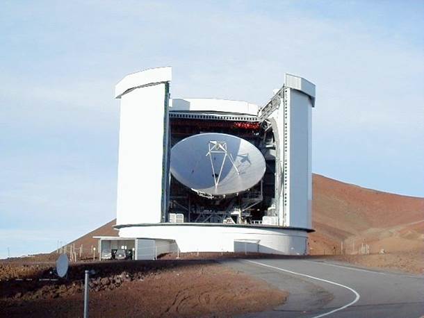
James Clerk Maxwell Telescope (JCMT) The 15-m James Clerk Maxwell Telescope (JCMT)was originally conceived and operated by a UK, Dutch and Canadian consortium. It is now operated by the East Asian Observatory. The telescope is situated near the summit of Mauna Kea in Hawaii at an altitude of 4,092 m; it has a surface accuracy of 24 μmr.m.s. enabling it to operate at sub-mm wavelengths (http://www.eaobservatory.org/jcmt/)

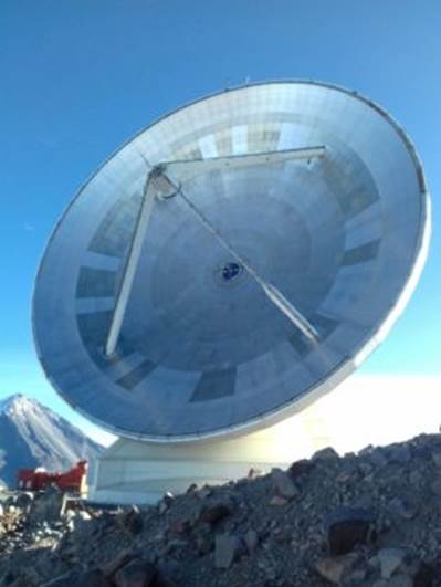
Large Millimetre Telescope The 50-m diameter Large Millimetre Telescope Alfonso Serrano is a Mexico/USA project situated on the summit of Volcan Sierra Negra at an altitude of 4600m. The primary surface was completed in December 2017. The LMT is now the world’s largest single dish designed for operation at short mm wavelengths. See http://www.lmtgtm.org/ and http://www.lmtgtm.org/13-december-2017-the-50m-diameter-primary-surface-completed/

Nobeyama 45m near Minamimaki, Nagano, Japan: the observatory is at an altitude of 1350m and the telescope was completed in 1982. It remains amongst the largest dishes aimed at mm-wave observations from 22-115 GHz and has made many contributions to radio astronomy. https://www.nao.ac.jp/en/research/telescope/45m.html

Mapping large areas of sky

The corrected Haslam 408 MHz all-sky map

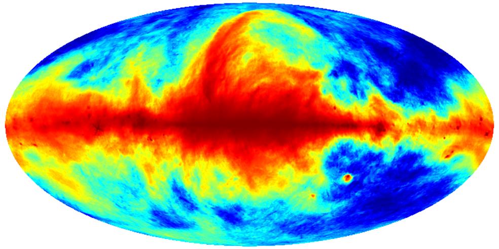
The classic 408 MHz all-sky map of Haslam et al (1982) (see Section 8.9) has been reanalyzed to remove residual errors. A full description of the processes involved is given in the paper: Remazeilles, M., Dickinson, C., Banday, A. J., Bigot-Sazy, M.-A., Ghosh, T., "An improved source-subtracted and destriped 408 MHz all-sky map", MNRAS 451, 4311 (2015).

Versions of the new maps can be downloaded from

http://www.jb.man.ac.uk/research/cosmos/haslam_map/

and

https://lambda.gsfc.nasa.gov/product/foreground/f_images.cfm

Sections of the 408 MHz all sky maps before (HAS03 an earlier version of the maps) and after correction (HAS14) taken from Remazeilles et al (2015). The stripes arose from total power (“baseline”) offsets principally due to receiver gain variations (“1/f noise”).

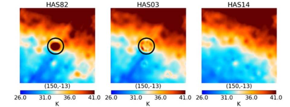
Discrete artefacts arose principally from imperfect subtraction of extragalactic sources. The source visible in HAS82 was imperfectly subtracted in HAS03 but well subtracted in HAS14.

References to other large area maps

Several other large area continuum surveys have been made with single dishes (see Remazeilles et al (2015) for references) while the HI4PI survey (Supplementary Material Chapter 3: Spectral Lines) is an all-sky spectral line survey. For references to other large area sky maps see Chapter 14.

Twin-beam Radiometry (Sections 4.4 and Section 8.6)

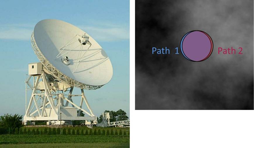
OCRA-p on the Torun 32-m dish

The 30 GHz OCRA-p radiometer, described in detail by Lowe (2006), and pictured in Supplementary Material Chapter 6, has twin feed horns and independent receivers and was mounted at the secondary focus of the Torun 32-m telescope (left hand panel); the front of the receiver housing can be seen just below the mouth of the square L-band horn. For large antennas (D > 15m) and at frequencies above ~10 GHz (λ < 0.03 m) the near-far field transition is more distant than ~15km (often much more) hence the path through the atmosphere is all within the near field. The right hand panel shows the two near-field beams (path 1 and path 2) projected on the sky with variations in the clear atmospheric opacity indicated via the gray scale. The beams largely overlap so rapidly differencing the receiver outputs (effected by a correlation-type receiver, see Supplementary Material Chapter 6) greatly reduces the atmospheric effects as well as receiver gain changes and changes in the ground spillover. Since twin beam radiometers differentiate the radio astronomical sky (the beams separate in the far field – see below) they are insensitive to slow angular variations in sky brightness. Reference: S. Lowe 2006 PhD. Thesis University of Manchester

Two beams above the atmosphere (in the far field)

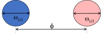
The overlapping “quasi-cylindrical “ near field patterns separate into the classical Fraunhofer beams with ≈1.2 λ/D - these beams do NOT overlap. Their separation φ= x/f where x is the separation of the feed centres and f is the focal length of the dish. Consider two cases:

a) Astronomical (not atmosphere) emission in both beams is very similar

· Constant background: thus [T_A1 -T_A2] = 0 hence no astronomical signal results.

· Taking the difference between the beams has “differentiated” the sky brightness temperature distribution - hence this method is insensitive to slowly varying T_B variations

b) Astronomical background emission is different in each beam

· Compact source in one and not the other

· System ideally suited for surveys or monitoring observations of compact sources

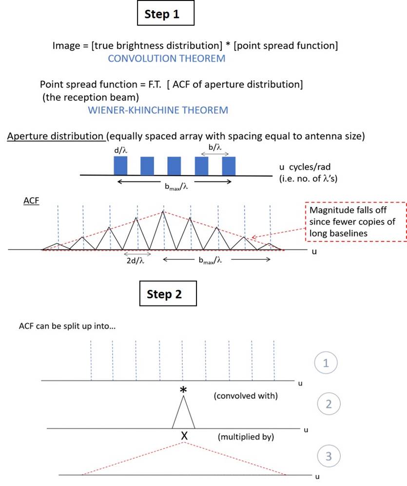
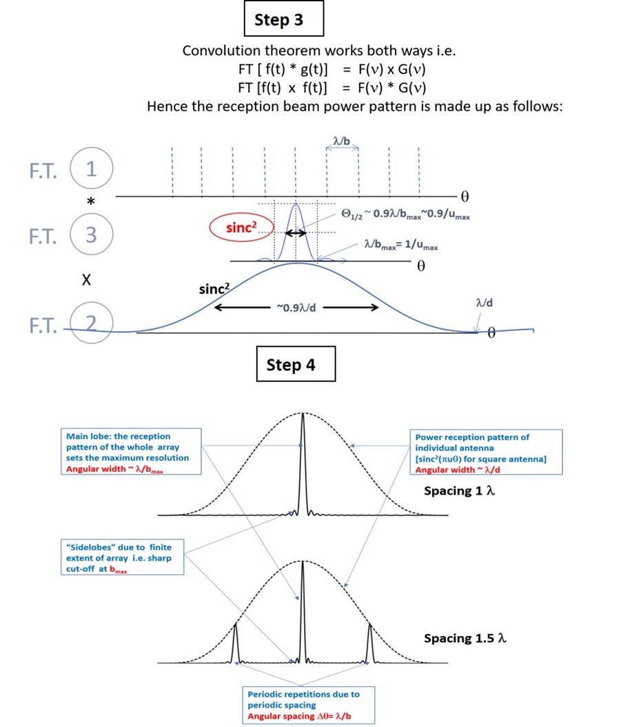
Phased array beam patterns – pictorial descriptions

Reception pattern of a simple phased array (adding beamformer)

Phased arrays provide “direct” imaging i.e. an instantaneous beam is formed just as in a single dish. The classic book “Radio Astronomy” by J.D. Kraus (section 6.4) provides a neat introduction to array theory although it is also covered in many other places. In our main text sections 8.2 and Fig8.11 we discuss the simplest case where all the array elements are connected to the same final receiver. In this case the relative weighting of the baselines is triangular (see also below). In the following set of diagrams we break down the formation of the beam into a series of steps

---N.B. antenna size is denoted by D in the main text not d as in the diagrams below--

The width of the primary beam and the height of the sidelobes can be altered with additional weightings/tapers. Appendix 6 of Kraus’s “Radio Astronomy” lists some standard tapers and the resulting beam patters which result.

Animations of phased arrays

There are many animations illustrating the basics of phased arrays available on the Web e.g. https://www.youtube.com/watch?v=vtPPAnvJS6c and https://www.youtube.com/watch?v=qvdfsgueJc8. The reader will be able to find others.

A illustration of the scientific advantages of a phased array can be seen by clicking mbrace.mp4 (credit M. Kramer). This animation schematically showcases the ability of the central block (implicitly containing many reception elements) to form multiple beams simultaneously – the number being limited only by the cost of the digital beamforming hardware. Many observers or groups of observers can therefore be running independent observations at the same time. At 00:00:06 the beam pointing to the right of vertical shows several higher resolution beams within it; this is the result of adding together data from the other blocks of elements around the central block. The upper panel in “Step 4” above shows one such “array” beam; additional array beams can be formed with more electronics. Also shown is the ability of a phased array to respond quickly to changes in the sky (appearance of transient sources).

Calibration of Single Dish Observations

The many practical issues of mapping calibration of single dish observations was not explicitly covered in Chapter 8 although some of the basic principles were covered and basic calibration principles were covered in Chapter 6. There are many sources of up to date advice and wisdom but a good place to start is the introductory paper:

“Single dish calibration techniques at radio wavelengths”: K O’Neil (2002) NAIC/NRAO School on Single-Dish Astronomy Techniques and Applications ASP Conference Series Vol 278 eds. Stanimirovic S., Altschuler D.R., Goldsmith P.F. and Salter C.J. also available at https://arxiv.org/abs/astro-ph/0203001

Other more detailed sources include:

The talks at NRAO Summer schools

https://science.nrao.edu/facilities/gbt/single-dish-school-lectures/sds-2015

https://science.nrao.edu/science/meetings/2015/summer-schools/single-dish-program

The European Single Dish School in the Era of Arrays https://www.mpifr-bonn.mpg.de/ESSEA2010

Broad band calibration for single dish telescopes: https://events.mpifr-bonn.mpg.de/indico/event/48/session/5/contribution/18/material/slides/0.pdf

Pointing single dishes

In section 8.9.4 we briefly discussed the pointing requirements of single dishes.    The paper “Green Bank Telescope: Overview and analysis of metrology systems and pointing performance”  by White et al.  https://arxiv.org/pdf/2111.12636.pdf describes in great detail the challenges overcome in pointing the world’s largest fully steerable single dish.