Supplementary Material to:

An Introduction to Radio Astronomy

4^th edition Cambridge University Press 2019

Last updated 1/07/2019

Chapter 7: Spectrometers and Polarimeters

Autocorrelation Spectrometers: revisited

Autocorrelation is most often used in the analysis of “noisy” data containing some suspected periodicities with low signal-to-noise ratio – this is just what a spectral line “buried” in system noise is – some frequencies contribute a little more power than others. The ACF is a measure of how predictable a function is at (t + τ) , i.e. a version delayed by τ, compared with the function at t. In Section 7.3 we outline the basis of practical digital autocorrelation spectrometers (ACS) but experience tells us that this process can be hard to understand at first sight. In this section we take a second look at how the ACF is formed from digitized data (see Appendix 3) with samples separated by time intervals t.

We start by outlining the most obvious approach (as in Section 7.2) which is not, in practice, used.

The TxN approach

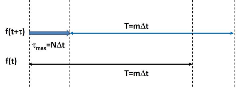
· As described in section 7.2 we start with f(t), comprising m samples over a time span T=mt and then:

o Cross-multiply, point by point, the m samples of f(t) with the m samples of f(t+τ) which have been shifted by a time τ [an integer number x sampling interval t].

o Adding up the results of the point-by-point multiplications over all T and averaging them together. This forms one point in the ACF.

o Repeating the process N times with increasing time shifts taking the total shift of f(t+τ) out to Nt = τ_max as in the diagram below. Note that N<<m.

o The number of digital operations is proportional to NxT

· This approach is like a digital version of a Michelson spectral interferometer; it effectively requires manipulating two extended data sets (in order to achieve the desired signal-to-noise ratio) plus the ability to cross-multiply them and add up the results for a set of delay steps (shifts or “lags”) to cover the range out to τ_max. It would require lots of specialised digital hardware.

In the practical numerical simulation shown in the diagram below (and also for a longer time series in Fig 7.3) N is not <<m and the decay (decorrelation) seen in the ACF magnitude is only due to the finite length of f(t) – which limits the extent of the overlap between the function and the shifted version (see the diagram above). This “window” limits the resolution of the retrieved frequency after Fourier Transformation. In a real observation decorrelation in the ACF also arises from the finite width of the spectral line. In the time domain a narrow spectral line is a quasi-sinusoidal signal which less and less resembles a time-shifted copy of itself; the decorrelation timescale is proportional to (1/linewidth).

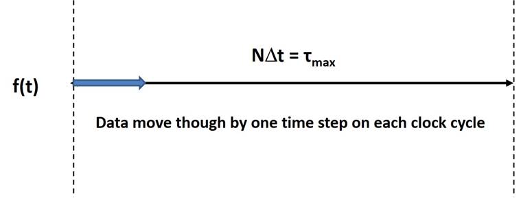
The NxT approach

A more practical approach involves reversing the order of N and T. Now one stores one continuously updated set of N samples f(t) covering the maximum time delay τ_max. Since N<<m the amount of data stored is much less than in the first approach. After each time step t the samples move along by 1 through the “window” (a digital delay line) defining f(t) i.e.

The ACF is formed by:

· Cross multiplying the first sample of f(t) with each of the other N samples in turn out to τ_max this gives an estimate of the complete ACF out to τ_max at one go. We are still seeing how the signal (albeit now only one sample of it) compares with shifted versions i.e. the other samples in f(t).

o Repeat the process after the next clock cycle i.e. multiply the new first sample with the others to form a new estimate of the complete ACF and add it to the first one. The signal-to-noise ratio of the co-added ACF will improve.

o Keep repeating the process for m clock cycles i.e. for an extended time period. With the same number of operations, proportional to (N x T), as in the first approach the ACF builds up to the same signal/noise ratio.

· Since we are working with many fewer data at any given time this method is more efficient in terms of digital electronics. It is used in all DACS.

Outline of the digital architecture (see also Fig 7.1)

· In the simplest digital system single bit samples (0,1) are fed into a digital delay line ( a “shift register“) storing the sampled input signal f(t) – out to N shifts (or “lags”)

· At a given time the state (0 or 1) of each stage in the shift register is compared to that of the 1^st(zero shift) stage. If both the same (0 or 1): comparator yields 1. If they are different the comparator yields 0; the result added into counter for each shift.

· On the next clock pulse all samples move along by one in the shift register and the process is repeated up to the chosen integration time (m time steps). The contents of the counters then form the sampled ACF.

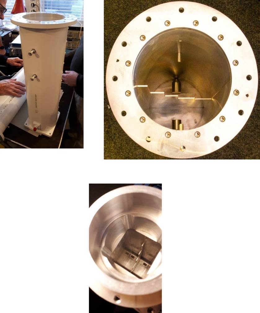
Septum plate polarization splitters

Septum plate polarizers (IRA4 Section 7.5). There are several ways to extract orthogonal polarizations from a symmetrical waveguide feed. The septum plate is widely used to produce the hands of circular polarisation due to its compactness, albeit at the expense of bandwidth. The top figure shows a septum polarizer in a circular waveguide optimized for the band 1400-1427 MHz (credit: Phase2 Microwave). The figure below shows a septum plate polariser in a square waveguide optimised for C-band operation – the section above the septum converts the waveguide cross-section from square to circular.