Supplementary Material to:

An Introduction to Radio Astronomy

4^th edition Cambridge University Press 2019

Last updated 1/07/2019

Chapter 6: Radiometers

Schematic illustration of the action of a mixer

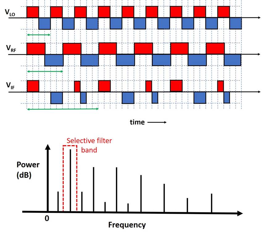
The essence of mixing is captured by the action of an “on-off” switch in which the conductance of a diode is controlled by the varying local oscillator (LO) voltage V_LO.

In the top panel the varying input LO and radio frequency (RF) and output intermediate frequency (IF) voltages are represented by square waves for simplicity. In the bottom panel the output spectrum of the intermediate frequency (IF) signal is shown.

Notes:

- In practice V_LO >> V_RF; ii) the LO frequency f_LO is shown as higher than the RF frequency f_RF but this is an arbitrary choice.

- When the LO voltage (period 4 units say equivalent to f_LO = “250 MHz”) is positive (red) the switch passes the RF signal (period 6 units equivalent to f_RF =“166.67 MHz”). When the LO voltage is negative (blue) the RF signal is not passed.

- The IF signal can be seen to have a component with a repetition period of 12 units equivalent to f_IF = “83.33 MHz” i.e. the difference frequency.

As can be seen, however, there are other frequency components in the IF signal and in practice a wide range of harmonics, and mixtures between them can be generated; this is shown schematically in an output spectrum in the bottom panel. The desired frequency component has to be selected out by a filter and the power in it is always significantly less that in the original RF signal; this is called the “conversion loss” and is typically in the range 6-10dB (see section 6.6).

Receiver Temperature Calibration

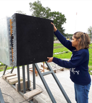
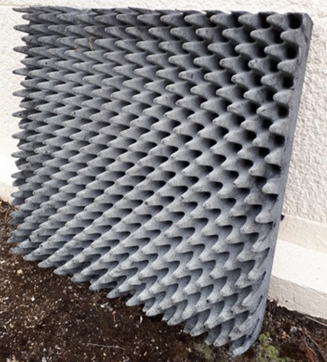
Measuring T_rec with a microwave absorber (IRA4 Section 6.5).The telescope aperture is covered with absorbing material (right) at ambient temperature, measuring the contrast between the (cold) sky temperature and the ambient temperature of the absorber.

In order to determine the receiver temperature output power measurements are taken for at least two sources of known input power. A sheet of carbon-loaded microwave absorber (top) radiates very like a black-body over a particular frequency range and is often used as the “hot load” at ambient temperature. A “cold load” can be created by soaking the absorber in liquid nitrogen (LN2) at a temperature of 77K. Here we show the absorber as a hot load being held over the mouth of an experimental corrugated test horn which is connected to a receiver. For the most accurate work the characteristics of the absorber must be precisely known at the observing frequency (from the manufacturer’s specification plus lab. bench measurements); the back of the absorber should be covered with reflecting material (a metal sheet) to double its effective depth. The temperature of the hot load must be measured at representative places and the known effect of atmospheric pressure on the boiling point of LN2 should be taken into account for the cold load. To achieve a lower temperature cold load liquid helium is used but the costs are much higher than for LN2.

For state-of-the-art discussions about precision total power calibration see:

C. Tello, T. Villela, S. Torres, M. Bersanelli, G. F. Smoot, I. S. Ferreira, A. Cingoz, J. Lamb, D. Barbosa, D. Perez-Becker, S. Ricciardi, J. A. Currivan, P. Platania, and D.Maino, “The 2.3 GHz survey of the GEM project”, A&A, 516, A1 (2013)

Singal, J; Fixsen, D.J; Kogut, A; Levin, S; Limon, M; Lubin, P ; Mirel, P; Seiffert, M; Villela, T; Wollack, E; Wuensche, C.A; 2011 “The ARCADE” Instrument”, ApJ, 730:138.

The universality of “1/f noise”

The appearance of 1/f spectra in a wide variety of natural phenomena has been discussed by, among others,

Milotti, E. (2002) https://arxiv.org/ftp/physics/papers/0204/0204033.pdf

Ward, L.M. and Greenwood, P.E. (2007) http://www.scholarpedia.org/article/1/f_noise

Schematic signal flow in a Dicke-switch system.

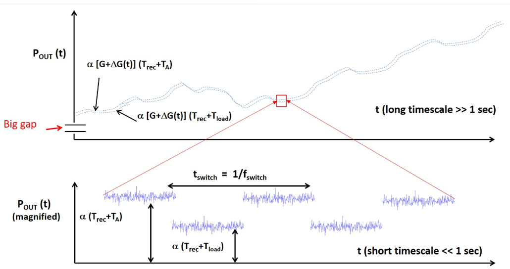
Schematic signal flow in a Dicke-switch system. In this receiver system (see Section 6.8.1) the noise power from an antenna is compared with that from a resistive load. The illustration shows the flow of signal through the system.

If the receiver gain fluctuations DG(t) were very slow (e.g. minutes) then one could calibrate a radiometer by frequently pointing the antenna at a sky reference region of known brightness. In practice the gain fluctuations (“1/f noise”) are much too fast for this approach and so in the Dicke switch system the comparison power source is built into the receiver itself in the form of a resistive load; the receiver input is switched between the antenna and the load (main text Fig 6.13). In the upper part of the signal flow diagram schematic output power fluctuations are shown for the case when T_A>T_load. The relative gain variations DG(t)/G have been greatly exaggerated by suppressing the steady (P₀) part of P_OUT (t); they are typically 1:10^-4 to 1:10^-5. If t_switch<< 1/f_knee the gain variations over a switching cycle will be small –akin to a fast shutter speed on a camera freezing the motion of a target. Note, however, that for ease of drawing t_switch is here only somewhat smaller than 1/f_knee rather than very much smaller. The lower portion of the signal flow diagram shows the power output for the two states P_out a (T_rec+T_load) and P_out a (T_rec+T_A) over a few switch cycles. The synchronous detector system responds to the average power difference a<T_load-T_A> rather than to the unswitched power a<T_rec+T_A> and thus the relative improvement in stability on the timescale of t_switch is [T_rec+ T_A]/ [T_load -T_A].

State-of-the-art Dicke-switch applications:

The advantages and disadvantages of Dicke switch receivers are described in the main text. They are used in accurate radiometers to measure atmospheric water vapour e.g. Tanner E.W. Radio Science, 33,449 (1998). Current high-profile applications are the 183 GHz water vapour radiometers for ALMA (Section 11.3) and the Earth resources satellites Aquarius (https://aquarius.nasa.gov ) and SMAP (https://smap.jpl.nasa.gov/mission/description/) which both use L-band radiometry demanding great precision and stability.

An example of a twin-beam radiometer: the 30 GHz OCRA-p system

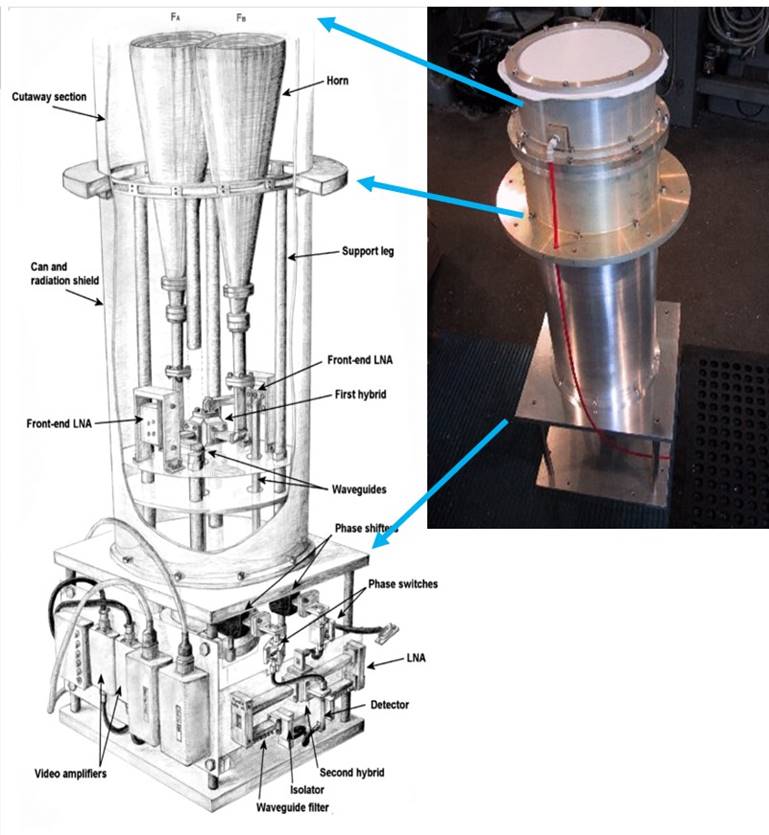
As explained in section 8.6.1 and Supplementary Material Chapter 8, a twin-beam receiver, which continuously takes the difference between the power in closely-spaced beams, greatly reduces the effect of tropospheric fluctuations, ground spillover and receiver gain changes. An example of such a system is the 30 GHz (λ = 1cm) OCRA-p radiometer (Lowe 2016 ; Lowe et al 2007) mounted on the 32m dish of the Torun Centre for Astronomy. In the drawing (left) the two corrugated horns (inner diameter at mouth = 80mm) feed power to a correlation receiver whose architecture is similar to that of the Planck LFI radiometers (see below and Chapter 17). The components (including the horns) above the horizontal plate are in a cryostat cooled to ~20K; below the plate the components are at ambient temperature. In the photograph (right) the receiver is shown prior to mounting on the telescope. The white material at the top is to prevent condensation forming on the microwave-transparent window (above the horns and not visible) which separates the atmosphere from the vacuum inside the cryostat. The red pipe feeds dry nitrogen into the space between the white material and the window to further reduce condensation on the window. (Drawing credit S. Lowe)

References

· Lowe, S.R. PhD Thesis, University of Manchester (2016)

· Lowe, S. R., Gawronski, M. P., Wilkinson, P. N., Kus, A. J., Browne, I. W. A., Pazderski, E., Feiler, R., and Kettle, D. 2007. 30 GHz flux density measurements of the Caltech-Jodrell flat-spectrum sources with OCRA-p. A&A, 474(Nov.), 1093–1100.

Schematic of a basic correlation receiver

Power from two closely-spaced beams (red and blue directions) enter the receiver and are continuously compared. The voltage outputs VA1 and VA2 (alternatively the comparison could be a temperature controlled load Vload) have, by means of the hybrid splitters, passed through both receivers and hence are subject to the same gain fluctuations. After square law detection the powers (TA1 and TA2 or Tload) therefore vary together and the difference TA1 - TA2 goes to zero if the receiver inputs are exactly balanced. When there is different emission in one of the beams (near field atmosphere or far field sources), this will appear in the difference signal. This is the essence of the OCRA-p architecture. In practice additional amplification is required after the second hybrid splitters and before power detection. Since the gain of these amplifiers will also vary an additional time modulation is applied in one arm between the splitters by means of 180^o phase switch. In a manner reminiscent of the operation of a DIcke switch system by subtracting the modulated signals the effect of the gain variations can be greatly reduced. This is shown in the schematic OCRA-p and Planck LFI radiometers below.

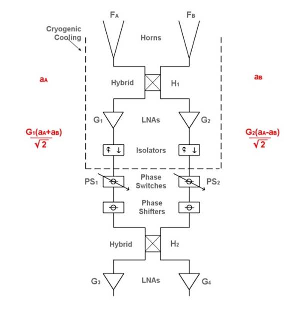
A schematic of the OCRA-p correlation receiver showing the phase switches between the two hybrid splitters. Only one of the phase switches is actually driven the other is in place to balance the characteristics of the two arms. The phase shifters allow small changes to the path length of the signal in the two arms to be made (Drawing credit S. Lowe).

A simplified picture of a Planck LFI receiver

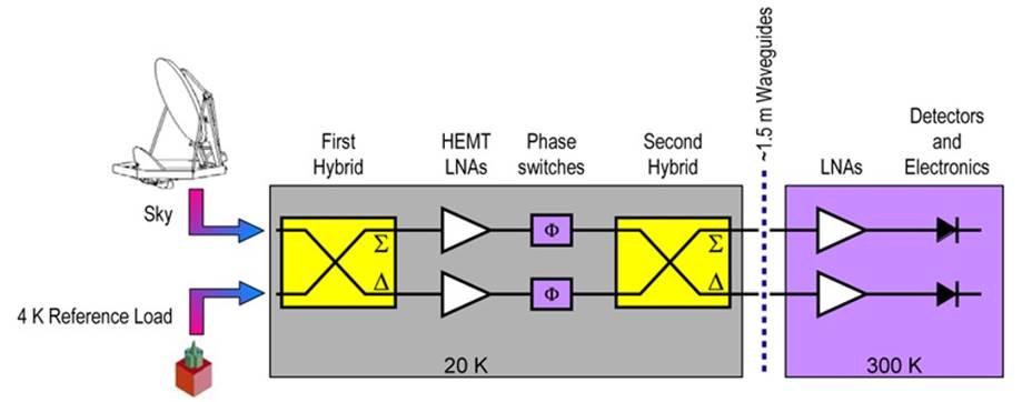
The Planck LFI receivers used thermal load as the reference since goal was to map extended CMB emission rather than discrete sources as in OCRA-p. Ideally the load would have been at the same temperature as the CMBR (2.75K) to balance the receiver and hence maximise the reduction in 1/f receiver gain fluctuations; the load was actually at 4K. Nevertheless the knee frequency was reduced from ~100 Hz to ~40 mHz (t ~ 25 secs) an improvement of 2500. Small non-modelled imperfections in component performance prevented a greater improvement. (Picture credit http://planck.caltech.edu/lfi.html )