Supplementary Material to:

An Introduction to Radio Astronomy

4^th edition Cambridge University Press 2019

Last updated 04/12/2021

Chapter 4: Radio Wave Propagation

Faraday Rotation

As described in Section 4.2 propagation through a magneto-ionic plasma rotates the plane of linear polarization of a radio wave. In the simplest case of a background radio source seen through a uniform cloud of thermal plasma threaded by a magnetic field the position angle is given by

where is the intrinsic position angle and the rotation measure (R radians m^-2) is defined in equation 4.10 (and see below). Typical values of R due to the ISM are in the range 1-100 rad m^-2 (see the discussion in section 14.10).

The pedagogic review paper “The Correct Sense of Faraday Rotation” by K. Ferriere, J.L. West & T.R. Jaffe  https://arxiv.org/pdf/2106.03074.pdf considers the effect of a magneto-ionic medium on linearly polarized synchtrotron radiation from first principles.  The conclusions are consistent with Section 4.2. There are, however, practical complications to the determination of rotation measures which we now sketch in.

There are, however, many complications to this simple picture which we now sketch in.

Rotation measure ambiguity

One can obtain a value of RM from just two measurements of the polarization angle (see equation 4.11) but this may well be incorrect since the polarization angle is only known modulo 180^o (i.e. radians) and one can add integer values of to the measured angle; this is known as the “n ambiguity”. The problem is best illustrated with a diagram.

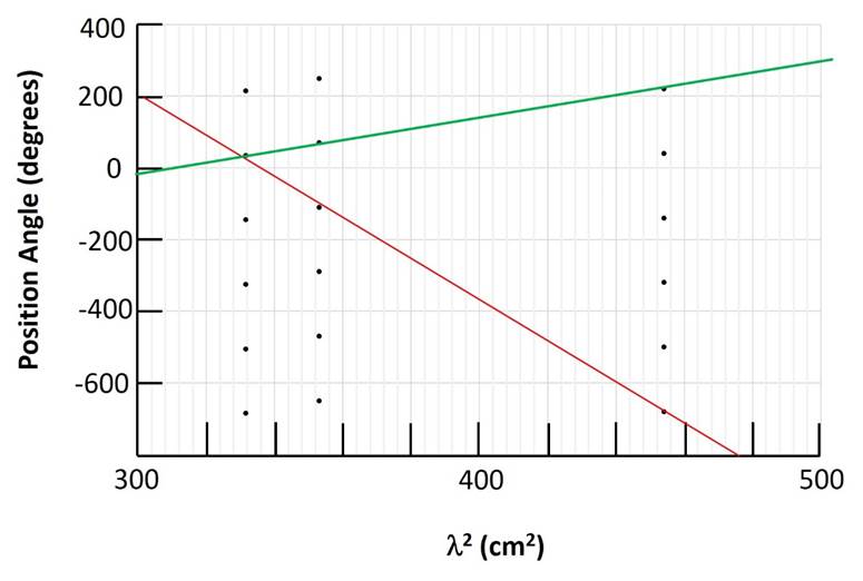
The plot above is a schematized version of Figure 1(b) in Rand & Lyne (1994). It shows the linear polarization angle (here given in degrees rather than radians) against λ² (here given in cm² rather than m²) of the radiation from a particular pulsar. A series of wavelengths in L-band were used for the observations but here we have plotted the results for only three wavelengths (~18.2 cm hence λ²=331.5 cm²; ~18.8 cm hence λ²=353 cm² ; ~21.3 cm hence λ²=454 cm²). The multiple possible value of polarization angle are shown for each value of λ². As Rand & Lyne (1994) discuss even with three wavelengths R is ambiguous since it is possible to plot two plausible straight lines through the range of possible polarization angles (R= 261 rad m^-2 (green) and R = -1006 rad m^-2 (red). Observations at additional closely-spaced wavelengths were required to reject the R=-1006 rad m^-2 alternative – see Rand & Lyne (1994) for details.

At the time of this update the most extreme rotation measure has been found in the repeating fast radio burst source FRB121102 (Michilli et al 2018) which has a R= ~1.4 x 10⁵ rad m^-2. The physical origin of the rotating medium remains unclear; but this value of R is orders of magnitude higher than can be ascribed to the ISM of the Milky Way.

Additional effects

The implicit assumption in the main text and the above discussion is that the Faraday Rotation is due to a uniform magneto-ionic medium which is itself not emitting or at least emitting much more weakly than the source under study. As broad-band polarization observations over extended emission regions become the norm these simplifying assumptions may not be valid. For example:

1. The source or region under study may consist of separate components with different spectral indices and intrinsic polarisations which can be blended together within the observing beam.

2. The thermal electron density and/or the strength and direction of the magnetic field in the intervening medium may vary significantly in depth and across the beam

3. The intervening medium may itself emit significantly, with different intensities and spectra, throughout its volume.

These effects were first systematically addressed by Burn (1966) and because of them:

a. The relationship between polarization angle and λ² along a given line of sight may not remain linear over a wide range of wavelengths.

b. At longer wavelengths, where the Faraday Rotation is larger, the total intensity along a given line of sight (within a beam) may decrease – this is “depolarisation”.

As a result there can be wide variations in the polarization observables across extended sources (see Section 14.10 in the case of the ISM).

Depolarisation

· If R is very high the rotation of the polarisation angle across a finite observing band can be large enough that the resultant signal is partially “quenched”.

· Cases (1 and 2) above can lead to external or “beam depolarisation” due the unresolved variations in polarization properties across the observing beam.

· Cases (2 and 3) amount to internal depolarisation in which the thermal magneto-ionic plasma is intermixed with relativistic synchrotron emitting electrons. In this case radiation

· from different distances (depths) are Faraday rotated by different amounts and the resultant polarisation is reduced.

As well as in the Galactic ISM these effects are manifest in extragalactic radio sources. One striking success of polarisation studies was the recognition (Garrington et al 1988; Laing 1988) that the differential depolarisation across the face of an extended double source is a strong diagnostic of its 3-D orientation with respect to the line of sight; the greater distance that the radiation from the receding (jet+lobe) has to travel results in greater depolarisation. This is the so-called “Laing-Garrington” effect mentioned in section 16.5.

Faraday Depth and Rotation Measure Synthesis

The discussion by Burn (1966) regarding the observational consequences of an admixture of rotating and emitting media extending over a finite depth has been extended by Brentjens & de Bruyn (2005) into a technique, known as Faraday Rotation Measure Synthesis; this can be used to dissect out the various contributions and resolve the “n ambiguity”.

The integral definition of Rotation Measure in equation 4.10 (with the integral often implicitly “solved” for the special case of uniform foreground slab – as above) was more generally interpreted by Burn (1966) as a “Faraday Depth” in order to encompass a distribution of Faraday rotating regions along a line of sight. Thus the more general Faraday depth is defined as in equation 4.10 i.e.

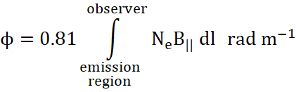
where integral over the path l (in pc) is along the line of sight to the emitting source; N_e is the electron density (in cm^-3) and B_|| is the component of the magnetic field (in microgauss) parallel to the line of sight. As noted by Brentjens & de Bruyn (2005) Faraday “screens” of extent can be characterised as “thin” in the case and as Faraday “thick” when .

In the general case the integral cannot simply be solved by inspection but the RM synthesis technique, coupled with polarization data over a wide frequency range, does enable the distribution of polarisation properties to be sorted out. The heart of the technique is the recognition that there is a Fourier Transform relationship between the observed complex polarization “vector” as a function of wavelength squared i.e. P(λ²) and the intrinsic polarized flux at a given wavelength. Reverting for the moment to the simplest case of a single source located behind homogeneous medium the observed polarization “vector” rotates uniformly as a function of λ²

Intrinsic polarized flux where I is the total intensity and p is the fractional polarization (see main text Section 7.5)

thus ;

and for the simplest rotated case ) ; )

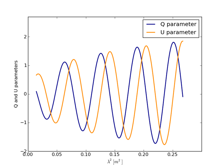
This case is illustrated in the simulated plot of Q and U below; note that the increase in magnitude with λ² is due to the steep spectrum of the model source flux density. [image credit: Simon Ndiritu]

In the time domain the analogy is the rotation of a vector in the complex plane of a single frequency sine wave signal. The Fourier Transform of a sine wave is a single point in frequency space which is then analogous to the single value of Rotation Measure. A general time varying signal is made up of (synthesized from) many sinewaves and hence, reversing the analogy, a general distribution of polarised emission and rotation measures adds up to (integrates to) the observed behavior of the polarized signal P(λ²). It can thus be imagined that the inverse Fourier Transform P(λ²) can, in principle, yield the intrinsic polarization behaviour along a given line of sight. For more details we recommend the reader starts with the tutorial by Heald (2008) before moving on to Brentjens & de Bruyn (2005). There are many papers illustrating the technique in action using modern broad band data; for example Ma et al (2019) resolved cases of the “n ambiguity” in NVSS sources while O’Sullivan et al. (2012) explored complex Faraday depth structure in AGNs.

References:

Brentjens M.A. & de Bruyn A.G. (2005), A&A, 441, 1217 (also https://arxiv.org/abs/astro-ph/0507349)

Burn, B.J. (1966) MNRAS, 133,67.

Garrington, S.T., Leahy, J.P., Conway,R.G. & Laing, R.A. (1988) Nature 331, 147

Heald, G., (2008) in Proc IAU Symposium no 259, p 591 (https://doi.org/10.1017/S1743921309031421)

Laing R. A., (1988), Nature, 331, 149

Ma Y.K. et al, (2019) MNRAS (in press) (also https://arxiv.org/abs/1905.04313v1)

Michilli et at (2018) Nature , 553, 182. https://arxiv.org/pdf/1801.03965.pdf

O’Sullivan, S.P. et al. (2012) MNRAS, 421, 3300.

Rand, R.J. & Lyne A.G. (1994) MNRAS, 268, 497

Scintillation

Dynamic frequency spectra observed from a pulsar

For a simple analysis of interstellar scintillation see Pulsar Astronomy, Lyne and Graham-Smith 4^th edn. 2012., or in more detail Walker M.A. et al 2008, MNRAS 388, 1214. This phenomenon is variable, depending on the changing structure of the ionised interstellar medium along and close to the line of sight. This can be studied through dynamic spectra, showing the effect of scintillation on a band of frequencies.

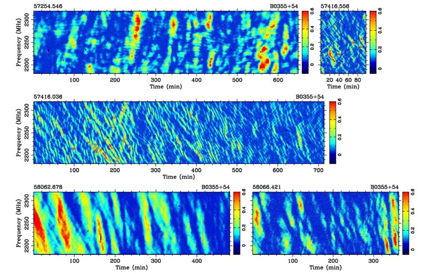
Dynamic Scintillation Spectra of PSR 0355+54 in five observations several months apart. Wang,P.F. et al https://arxiv.org/abs/1808.06406

The shape of the scintillation pattern on the earth’s surface surface has been explored using VLBI, and it now appears that scintillation is best explained by refraction at low angles of incidence on a small number of plasma sheets along the line of sight (Brisken W.F. et al 2010, Ap J 708,232.). Further evidence is found in the detail of the ‘scintillation arcs’ observed in the secondary spectra obtained by a two-dimensional Fourier analysis of the dynamic spectra. See a recent review by Stinebring D.R.2017 Proc IAU Symp 337, 287.

Solid angle of Mars from optical telescope measurements

Disk diameter = 24.8 arcsec

Diameter = 24.8/206265 = 1.20 x 10^-4 radians

(180/p).60.60 = 206265 arcseconds per radian

Disk area = pD²/4 = p [1.20 x 10^-4]²/4 = 1.135 x 10^-8 rad²

à W_MARS = 1.14 x 10^-8 rad² (or sterad)