Supplementary Material
to:
An Introduction to Radio Astronomy
4th edition Cambridge University Press 2019
Last updated 4/12/2021
Chapter 11: Further Interferometric
Techniques
Interferometer
Arrays at mm wavelengths
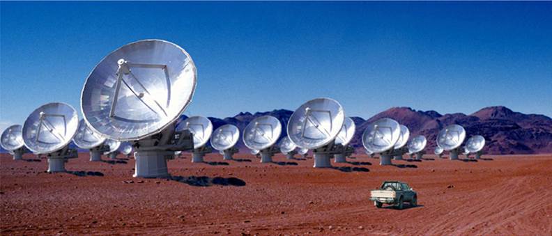
ALMA:
the Atacama Large Millimetre Array is located on the Llano de Chajnantor in Chile at an altitude of5000metres; its receivers cover
bands in the frequency range 84-950GHz. The main array comprises 50 × 12-m antennas which can be moved into different configurations
from compact (baselines to 150m) to extended (baselines to 16 km). The Atacama
Compact Array (ACA) is a subset of four 12-meter antennas and twelve 7-meter
antennas which are closely separated to improve ALMA’s ability to study objects
witha large angular size. www.almaobservatory.org/
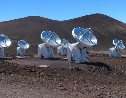
SMA:
the Smithsonian Submm-wave Array on Mauna Kea, Hawaii (altitude
4080metres) has 8×6-m antennas which can be configured
to provide baselines up to 783m. The receivers cover the wavelength range 1.7
to 0.7 mm (180-418GHz) in three bands. www.cfa.harvard.edu/sma/

NOEMA: the Northern Extended Millimetre Array of the Institut de Radio Astronomie Millimetrique is located on the Plateau de Bure in the French Alps (altitude 2550metres). When completed in 2019 it will have 12 × 15-m antennaswhich can be moved on E-W and N-S tracks to provide baselines up to 760m. (The image shows the 6 original antennas in an extended configuration). Four suites of receivers cover atmospheric windows from 3mm to 0.8mm (72-373GHz). http://iram-institute.org/EN/noema-project.php
Interferometer
Arrays at Long wavelengths

LOFAR: the
international Low-Frequency Array is centred in the Netherlands (maximum
baselines ∼100 km)
with (in 2017) external partner stations in Germany, France, UK, Sweden, Poland
and Ireland (maximum baselines1500 km). It operates in two bands: LOFAR-low
(10-80GHz) uses low-cost droop dipoles; LOFAR-high (120-240GHz) is built up from ”tiles” made up from 4×4 bowtie
dipoles (Section 8.1.3). A typical station consists of 96 low-band antennas and
48 high-band antenna tiles. There are 18 ”core”
stations and 18 ”remote” within the Netherlands and (currently) 8 international
stations. Each ”station” can produce one or more beams
which can be cross-correlated with the equivalent beams from other sites to
form an aperture synthesis array. The latter system relies on broad band
optical fibre data links with the digital correlation carried out via software in
a high performance computer rather than in purpose
designed electronics. www.lofar.org/
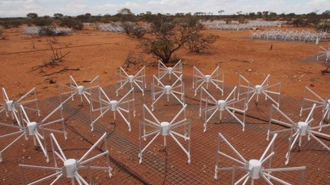
MWA: the
Murchison Widefield Array
is located in Western Australia near the plannedsite
of the SKA-low telescope. It consists of 2048 dual-polarization bowtie dipoles
(Section 8.1.3) optimized for the frequency range 80-300MHz. As in LOFAR-high
they are arranged in tiles of 4×4 dipoles
giving a field of view of 25◦at 150MHz. The majority of the
original 128 tiles are distributed
within a ∼1.5 km
core region so as to provide high imaging quality at a resolution of several
arcminutes. A phase 2 expansion which doubled the number of tiles to 256 (and
the number of dipoles to 4096) was commissioned in April 2018 http://www.mwatelescope.org/telescope.
An update
on the status and performance of the MWA can be found at:
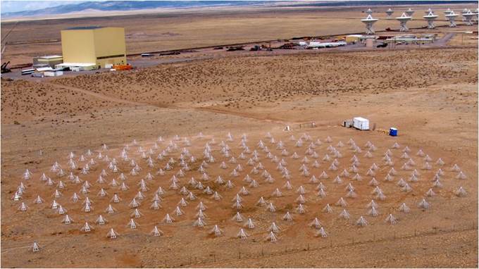
LWA:
the
Long Wavelength Array has been developed by the University of New Mexico and a
consortium of US partners. There are two sites: in New Mexico close to the JVLA
(run by University of New Mexico) and in Owens Valley California (run by
Caltech). At each site there is
currently a single ”station” consisting of 256
linearly polarized crossed dipole elements distributed over a 100 m diameter
area and sensitive to the frequency range 10-88 MHz (New Mexico) and 27-85 MHz
(0wens Valley). http://www.phys.unm.edu/~lwa/index.html and http://www.tauceti.caltech.edu/LWA/
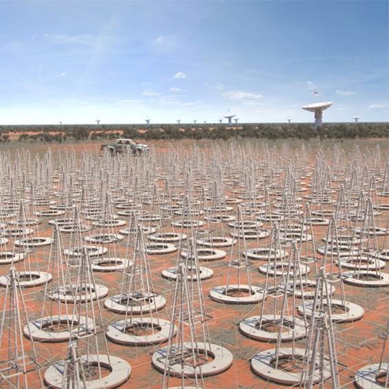
SKA1-low: (artist’s
impression)The SKA low frequency aperture array (LFAA)
will be located in Western Australia and is designed to cover the frequency
band 50 – 350 MHz. It will consist of ~130,000 fixed
antennas spread between ~500 stations with a maximum distance between stations
of 65 km. At the lowest frequency its total collecting area will be ~0.4 km2
https://www.skatelescope.org/lfaa/
Very Long Baseline Interferometer Networks
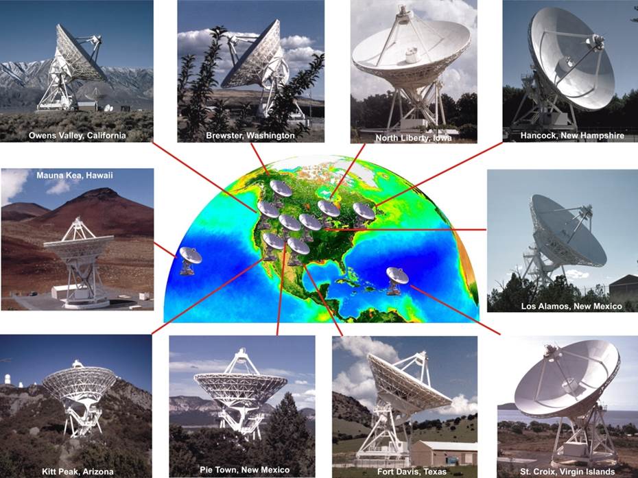
VLBA: the Very Long Baseline Array of the
USA is a dedicated facility consisting of 10 × 25-m
identical telescopes. Their locations extend at northern latitudes from New
Hampshire to the state of Washington, and at southern latitudes from St Croix
in the Virgin Islands to the island of Hawaii.The
central correlator is located at the NRAO Science Operations Centre,Socorro, New Mexico. www.science.nrao.edu/facilities/vlba

EVN: The European VLB Network is a
cooperative arrangement of radio telescopes in the UK, Netherlands, Germany,
Italy, Poland, Russia, Ukraine, China and Japan with other antennas joining
from time to time. The central correlation facility is the Joint Institute for
VLBI in Europe (JIVE) at Dwingeloo, The Netherlands.
Periodically the EVN and the VLBA cooperate to form a world-wide network. At
the time of writing the EVN operates in real-time fibre-connected mode for ∼25% of the total time allocated for
EVN operation; this percentage will grow with time. www.evlbi.org/

East Asian VLBI Network the Japanese VLBI Network (JVN) and the Japanese dedicated
astrometric array (VERA) with its dual-beam antennas work independently. VERA
will also work in cooperation with the Korean VLBI Network (KVN) to form the kaVA.
www.miz.nao.ac.jp/en/content/project/east-asia-vlbi-network
and https://radio.kasi.re.kr/eavn/main_eavn.php
Australian
VLB Array: consists of the Australia Telescope Compact Array and single
dishes at Parkes, Tidbinbilla, Hobart Ceduna and Perth.
It is the only VLBI array in the southern hemisphere www.atnf.csiro.au/vlbi/
IVS: the
International VLBI Service for Geodesy and Astrometry coordinates global VLBI
resources for positional VLBI. At various times this includes 45 antennas
sponsored by 40 organizations located in 20 countries.The IVS Coordinating Center
is located at Goddard Space Flight Centerin
Greenbelt, MD. The next generation coordinated facility ”VLBI2010”
is planned to have more small fast-slewing antennas and a much enhanced multi-band
receiving system https://ivscc.gsfc.nasa.gov/
GMVA: The
Global mm-wave VLBI Array is a cooperative arrangement of many mm-wave
telescopes under the auspices of five different internationalorganisations.
They come together about twice per year to make coordinatednetwork
observations.
https://www3.mpifr-bonn.mpg.de/div/vlbi/globalmm/
EHT: the Event
Horizon Telescope https://eventhorizontelescope.org is another
international coordinated network of independent telescopes, it includes the
phased-up ALMA. The purpose is to make ultra-high resolution
observations at 1.3mm wavelength with a particular target being the massive
black hole at the centre of the Milky Way and the giant elliptical galaxy M87. In April 2019
the EHT consortium published the first images showing the “black hole shadow”
of the SMBH in the nucleus of M87 – see references and further details in Supp.
Mat. Chapters 9, 11 & 16.
Space
VLBI
VSOP/HALCA:
was
the first dedicated space VLBI project . The 8-m
antenna was launched by Japan’s Institute for Space and Astronautical Sciences
in 1997 and operated until late 2005. The orbit took the antenna from 12,000 to
27,000 km above the Earth’s surface providing resolutions about 3 times higher at a given wavelength than Earth-based
arrays. https://science.nasa.gov/missions/halca
RadioAstron: http://www.asc.rssi.ru/radioastron/
is the second dedicated
space VLBI project led by the Astro Space Center of
the Lebedev Physical Institute in Moscow, Russia. The spacecraft was launched
in July 2011 and operated until January 2019. The reflector is 10m in diameter
and the orbit takes it out to 350,000 km from the Earth thus providing
resolutions > 30 times those available in Earth-based arrays. A review of
the role of RadioAstron in AGN studies is given by
Bruni et al (2019) https://arxiv.org/abs/1904.00814
Gurvits (2019) has reviewed the history of space VLBI from concepts to
operational missions: see https://arxiv.org/abs/1905.11175
Special
purpose arrays
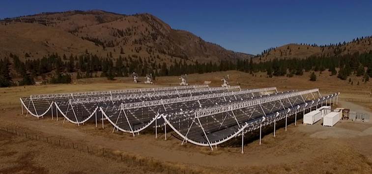
CHIME The Canadian Hydrogen Intensity Mapping
Experiment is located in Penticon, British Columbia
Canada. It consists of four adjacent 20m x 100m cyclindrical
reflectors orientated north-south. The focal axis of each cylinder is lined
with 256 dual-polarization antennas covering the frequency range 400-800 MHz
and giving it a very wide field of view. Its main targets are baryon acoustic
oscillations (BAO) which are diagnostics of Dark Energy and sources of Fast Radio Bursts
(FRBs). An outline explanation of
the experiment and of its beamforming and image formation capabilities can be
found at: https://chime-experiment.ca/.
HERA The Hydrogen Epoch of Reionization Array is designed for a frequency range 50-225
MHz to observe large scale structure at epochs around the Epoch of Reionization.
It will consist of 331 x 14 meter diameter non-tracking dishes pointing vertically
and packed into a hexagonal grid 310 m in diameter. HERA is
being constructed in the Karoo desert of South Africa with completion expected
in Q4 2020 see https://reionization.org/
HIRAX The Hydrogen Intensity and Real-time Analysis eXperiment aims to map the southern sky in continuum and
redshifted neutral hydrogen emission in the band 400-800 MHz to look for baryon
acoustic oscillations (BAO) which are diagnostics of
Dark Energy and sources of
Fast Radio Bursts (FRBs). It will
consist of ~1000x 6m non-tracking dishes and will be located in the Karoo
desert of South Africa; see https://www.acru.ukzn.ac.za/~hirax/
TIAN-LAI The
Tian-Lai Project is situated in north west China and is aimed at using 21cm
intensity mapping to detect baryon acoustic oscillations see http://tianlai.bao.ac.cn/
Techniques
in Aperture Synthesis: resources
Spectral Lines
http://www.astron.nl/eris2017/Documents/ERIS2017_L11_Johnston.pdf
Polarisation
http://www.astron.nl/eris2017/Documents/ERIS2017_L13_Marti-Vidal.pdf
Millimetre wave interferometry
http://www.astron.nl/eris2017/Documents/ERIS2017_L6_Pietu.pdf
Mosaicing:
Detailed
discussion of practicalities : https://science.nrao.edu/facilities/vla/docs/manuals/obsguide/modes/mosaicking
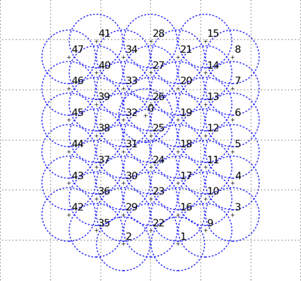
A set of pointings to cover a large field of view
The circles
represent the FWHM of the antenna primary beam (all identical) and the pointing
centres are separated by 0.5 FWHM. A
central beam e.g. number 25 is surrounded by a hexagonal pattern of beams
18,24,31,32,26,19. Another example is
the beam number 10 surrounded by beams 11,4,3,9,16,17. A mosaiced image made with such a pattern is
shown in Supp. Mat. Chapter 16 under “Faint Radio Sources” (courtesy T. Muxlow).
Filling in
short spacings with single dish data
These two presentations
both have illustrations of using a single dish to fill in lack of short
spacings in correlation interferometers
https://www.atnf.csiro.au/research/radio-school/2017/lectures/west-single-dish-astronomy-2017.pdf
VLBI
https://science.nrao.edu/science/meetings/2018/16th-synthesis-imaging-workshop/talks/Deller_VLBI.pdf
http://www.astron.nl/eris2017/Documents/ERIS2017_L12_Campbell_no-anim.pdf
version with animations:
http://www.astron.nl/eris2017/Documents/ERIS2017_L12_Campbell_with_anim.pdf
Wide-field
imaging:
https://science.nrao.edu/science/meetings/2018/16th-synthesis-imaging-workshop/talks/Rao_Wide_1.pdf
https://science.nrao.edu/science/meetings/2018/16th-synthesis-imaging-workshop/talks/Rao_Wide_2.pdf
http://www.astron.nl/eris2017/Documents/ERIS2017_T9A.pdf
Update on the ICRF3 and link with Gaia
“The third realisation of the international celestial reference frame by very long
baseline interferometry” has been published
by Charlot et al https://arxiv.org/abs/2010.13625. It contains positions for 4588 compact radio sources. A
subset of 303 sources, uniformly distributed on the sky, are identified as
"defining sources" and as such serve to define the axes of the
frame. A subset of 500 sources is found to have extremely accurate
positions at 8.4 GHz, in the range of 0.03 to 0.06 mas. Comparing ICRF3 with
the Gaia Celestial Reference Frame 2 in the optical domain, there is no
evidence for deformations larger than 0.03 mas between the two frames.
New
astrometric applications in the Solar System

An exciting new application of VLBI astronomy is in the
Solar System. Here VLBI
observations provide not only celestial 2D coordinates but can take advantage
of ultra-precise radial Doppler measurements of spacecraft, down to the
residual noise of ~0.015 mm/s. The technique is called PRIDE - Planetary Radio
Interferometry and Doppler Experiment. The tracking of the Huygens lander (part
of the Cassini mission) onto Titan on 14 January 2005 was the first
demonstration of PRIDE. The picture shows an artist’s impression of the Huygens
probe arriving at Titan together with the reconstructed descent trajectory of
the probe. The latter is based on various in-situ measurements with the
on-board instruments (cameras, altimeters, accelerometers) and VLBI tracking of
the probe at 2040 MHz with a network of 17 radio telescopes distributed
globally (Asia, Australia, Europe and USA). VLBI tracking provided the highest
lateral (astrometric) precision of 1 km (1-sigma) in the ICRF frame.
Currently the working goal of PRIDE is a 1-sigma lateral precision of ~50 m at the 5
A.U. distance of the Jovian system using observations at X-band (8.4 GHz). (Credits: Artist’s
impression – ESA and D.Ducros;
Descent trajectory – Huygens DTWG and JIVE (Leonid Gurvits)).
As well
as ultra-precise astrometry of spacecraft and natural celestial bodies in Solar
System future applications of PRIDE include: improvements of planetary
ephemerides, detection of Solar Coronal Mass Ejections, measurements of
planetary atmospheres (e.g. Venus, Mars) by means of radio occultations,
verification of the Einstein Equivalence Principle. Recent references to the astrometric
technique are:
D. A. Duev et al 2012,
“Spacecraft VLBI and Doppler tracking:
algorithms and implementation” A&A, 541, A43
D. A. Duev et al 2016, “Planetary
Radio Interferometry and Doppler Experiment (PRIDE) technique: A test case of
the Mars Express Phobos fly-by”, A&A 593, A34.
Geodesy
An Introduction/Overview
VLBI has made major contributions to the study of plate tectonics. A useful introduction can be found at
A publicly available 50+ page tutorial document on geodetic and astrometric VLBI (Elements of Geodetic and Astrometric Very Long Baseline Interferometry)
written by Axel Nothnagel can be found at https://www.vlbi.at/index.php/rushmore_teams/axel-nothnagel/. He states that this document is an open tutorial for educational purposes, in particular for newcomers to geodetic and astrometric VLBI but also for the specialists wanting to expand their knowledge about topics, which are not in their main focus.
Increasing separation of a
transatlantic baseline

A baseline between Europe and the USA is lengthening at 17.28 ±
0.16 mm per year. The plot above shows
the change in baseline length measured between radio telescopes at Westford (MA, USA) and Wettzell (Germany). Each dot represents
the 24h-average length of the baseline determined with a single VLBI session.
The observations are X- / S-band group delays taken from the IVS (International
VLBI Service for Geodesy and Astrometry) archive; the errors are obtained by
propagation of the formal errors of the geocentric coordinates. The long-term change is caused
by a superposition of plate tectonic and inter-glacial isostatic adjustment
processes, which are different at the two sites. In addition to the long-term
change, the original data show a faint quasi-sinusoidal variation. This signal
originates from displacements of the crust due to geophysical surface loading -
mainly of hydrological, atmospheric and oceanic origin - that are currently not
considered as conventional analysis models (IERS Conventions). The deviations
are more pronounced prior to about 1994 when the networks of IVS observing
stations customarily contained small numbers of antennas (> 5) and the
observation quality was not as good as it is today (image courtesy Robert Heinkelmann and
Susanne Lunz
GFZ Potsdam - see
Update on the
World-wide geodetic array: VLBI2010
Plate motions are now studied
predominantly with GPS and so the main scientific thrust of VLBI geodesy is the study of the
Earth’s rotation which requires comparison with the fixed quasar reference
frame ICRF2 and ICRF3. GPS from orbiting
satellites is not suited to Earth Rotation studies.
The international IVS service is engaged in a major upgrade to the world-wide geodetic array. This includes new 14m telescopes with fast slew speeds and instantaneous broad band receiving systems (2-14 GHz) see https://www.mpifr-bonn.mpg.de/1263600/Hase_110329VLBI2010.pdf
The
SMOS Earth Resources Satellite

The
European Space Agency’s SMOS satellite (see https://earth.esa.int/web/guest/missions/esa-operational-eo-missions/smos/multimedia-book) is a radio telescope in space pointing
downwards; it operates on the same interferometric principles as, for example,
the JVLA with which it shares the Y-shaped antenna array configuration. SMOS
operates at L-band where the atmosphere highly transparent and by detecting small changes in surface brightness
temperature measures soil
moisture, sea surface salinity, sea ice thickness and others geophysical
variables (image credit European Space
Agency).
Note that the NASA/JPL/GSFC single dish radiometer missions
Aquarius and SMAP share the same observational goals (see Supp. Mat Chapter 8)
as SMOS. All these missions demand
highly accurate (0.1K) calibration of surface brightness.
Pros and
cons of single dishes vs. phased arrays vs. aperture synthesis arrays:
Single dishes:
Scientific
Advantages: where the angular resolution of the dish does not matter
• Searching for pulsars
and timing them (Sections 15.13 & 15.16) – with the aid of focal plane
arrays or PAFs
•
Searching for Fast Radio Bursts (new Supp.Mat. section “The Time Variable Radio Sky”)
•
Involvement in VLBI Networks –
resolution then set by antenna separations (Section 11.4)
Scientific
Advantages: where the filled aperture of the dish matters
•
Large-area spectral line and continuum surveys - no
low brightness emission is missed
(Chapter 14) also low
angular resolution means sky can be mapped in a practical period of time.
Technical
advantages
• Receiver systems: are usually one-off designs
and hence relatively easy to change/upgrade
•
Standard
methods for observations/analysis developed over decades.
General disadvantages
•
Size and
collecting area limited:
-
sensitivity limited
-
angular resolution limited: hence cannot localize FRBs
and also source
confusion limits deep surveys (Section 8.9)
- accurate power calibration difficult (Section
6.5 and Supp. Mat. Chapter 6)
• Greater susceptibility to unwanted signals
(RFI, see Section 1.5 ).
See also
the presentation: https://www.mpifr-bonn.mpg.de/948285/Possenti_Why_Single_Dish.pdf
Adding interferometers (beam-forming arrays; phased arrays; aperture
arrays):
General points
o Adding responses produces “direct” imaging - form an instantaneous power
beam like single dish (Section 8.2; section 11.6; Supp Mat Chapter 8).
o Flexible digital beam forming enabled by the on-going revolution in
digital signal processing
o Higher sidelobes in “tied array beams” (Section 8.2; Supp
Mat Chapter 8) arise from an unfilled aperture; but
reducing the maximum baseline to get better instantaneous filling limits
the resolution.
o The number of elements required to cover a given
area increases as (wavelength)-2 thus costs currently set the upper frequency limit (for large areas) at about 350 MHz with dipole-like elements
(section 8.1; section 11.6); technology improvements required for dense aperture
arrays at higher frequencies.
Advantages
· Well-suited for real-time “non-imaging” applications e.g. pulsars and transients too small to resolve
and for which precise amplitude calibration is less important than for
synthesis imaging
· With independent delay systems can populate the primary beam of individual
elements or patches with many higher resolution “tied array beams” (Section 8.2)
thus particularly good for surveys for transient sources.
Disadvantages
o Subject to receiver gain variations, just as single dishes
o To cover the antenna primary beam with “tied array” beams likely to
require a major investment in electronics
o
Pose a calibration challenge for wide-fields and long integrations: (Section 11.6)
§
Difficulty in
characterizing the element primary beam, on all baselines
§
At long wavelengths
and long baselines: suffer the effects of the turbulent ionosphere (section
4.4; section 9.7; section 11.6)
Multiplying or
correlation interferometers (aperture synthesis arrays):
General points
·
“Indirect” imaging: spatial coherence (section
9.6) i.e. visibility data are in the Fourier domain – image reconstruction is a
secondary step. Compare with
i)
X-ray crystallography: which only measures the intensity of the
scattered waves and does not have direct access to the Fourier phase as in
radio interferometry; also uses “tricks” to obtain phase information.
ii)
Holography:
where phase information is
partially captured via intensity fringes in the hologram formed by adding the
scattered wave with a reference wave.
· Can assemble large
collecting areas from many smaller elements (Chapter 10) with resolution set by
the antenna separation not the size of the antennas.
· In contrast to adding
arrays correlation arrays see the entire field-of-view, set by the primary
antenna beam, at once.
Advantages
·
Correlating the complex electric fields gives access
to relative phase
information
o provides positional accuracy well within the conventional synthesised
beam for astrometry and geodynamics (Section 9.3; Section 11.4)
· Confusion limit much
lower than for single dishes: higher resolution means less blending of the
responses to the population of discrete sources (Section 10.12).
·
Resistant to uncorrelated signals
o
Gain variations in independent receivers
o
Atmospheric emission above independent antennas
o
Less sensitive to man-made RFI than dishes
Disadvantages
·
Only
N(N-1)/2 baselines thus the Fourier transfer function has gaps
o Deconvolution techniques usually required to
“fill in the gaps” but with no formal guarantee of the fidelity of the
reconstructed image (section 10.15)
o No “zero-baseline” information (section 11.5)
and finite filling factor gives reduced brightness temperature sensitivity
(section 10.12) hence not well suited to imaging smooth low brightness emission
o In worst case (typically wide fields and low
frequencies) visibility information collected may be insufficient to capture
the complexity of the field being imaged.
- Indirect imaging: is, in principle, not well-suited for real-time study of rapidly
time-variable sources e.g. pulsars and FRBs. However
this situation is constantly changing as digital data processing gets
faster and cheaper. For example:
- Buffering of digital
data now allows for a posteriori detection
and study of time-variable sources detected incoherently; recent examples
of the technique are described by Bannister et al (2019) https://arxiv.org/abs/1906.11476 using the Australia Telescope SKA Pathfinder (ASKAP) and by Ravi et
al (2019) https://arxiv.org/abs/1907.01542 using the Caltech Deep Synoptic Array
prototype.
- The CHIME array creates 4x 256 beams
using the Fast Fourier Transform (e.g. http://www.ursi.org/proceedings/procGA17/papers/Paper_J33-2(2946).pdf ) currently (2019) with a cadence 0.983 millisec.
- A spatial FFT-based approach to
handling the data from an array removes the needs for cross-correlation
of antenna pairs to synthesise an aperture (e.g. M. Tegmark & M. Zaldarriaga,
2008, Phys. Rev. D, 79,
8 available at https://arxiv.org/pdf/0805.4414v2.pdf. ) An
implementation of this technique on the Long Wavelength array has the
goal of real all-sky imaging at 50
millisec time resolution https://arxiv.org/pdf/1904.11422.pdf.
Routes to survey speed improvements
Survey Speed ~ [Aeff/Tsys]2
x BW x FoV
· Effective area: Aeff
o Invariably at a
cutting edge since natural radio sources are very weak
o For dishes the size
is fixed at build time but the feed illumination pattern (Section 8.3) can be optimised with phased array feeds (Section 8.7) à limited
improvement possible
o For
arrays can always add more elements
· System temperature: Tsys
o Receiver performance
is already close to realistic limits – particularly from ground-based sites à only limited
improvement possible in Tsys (Section 6.4)
·
Receiver frequency bandwidth: BW
o Can use broad-band
single pixel feeds (Section 8.1) for dishes and arrays but the practical
frequency range is limited by need to maintain polarization purity across the
band (section 7.6) and RFI.
·
Field-of-View: FoV
o
Sky coverage of single dishes increased with focal
plane horn arrays and phased array feeds (PAFs) à major improvement
possible in FoV (Section 8.7); the cutting edge is now
the development of cryogenic PAFs.
o
Arrays can take advantage
of PAFs – current examples are ASKAP and WSRT/APERTIF (Section 8.7; Section 10.1
and Supp. Mat Chapter 8).
o Low frequency arrays with small basic elements are already sensitive to
huge areas of sky (Section 11.6).
The
Square Kilometre Array
The SKA public web site
The SKA public web site https://www.skatelescope.org/ provides comprehensive overview of all aspects of the project to build the world’s largest radio telescope, at sites in Africa (South Africa initially) and Australia. The Global Headquarters of the SKA Organisation is at the Jodrell Bank Observatory UK which is the scientific home of two of the authors (FGS and PNW).
The first four sections:
· About the SKA
· Design
· Technology
· Science Goals
contain most of the material which directly complements our text although the other sections are also full of interesting information, in particular more detailed technical information and memoranda. The reader should browse them at leisure. As regards the sections listed above we draw particular attention to following sub-sections
· About the SKA
o The SKA Project
§ The layout
o The specific sites in Africa and Australia
· Design
o The work of the nine international consortia which came together to design the first phase SKA1 which will be built
o The advanced instrumentation programme looking ahead to technology enhancements in particular
§ Wide Band Single Pixel Feeds;
§ A mid-frequency aperture array;
§ Phased array feeds.
· Technology
o Aperture arrays (SKA1-LOW in the first instance)
o SKA dishes
o Software and computing
o Signal processing
o Precursors and Pathfinders (ASKAP; MeerKAT; MWA; HERA)
· Science Goals
o Concise descriptions of the SKA’s Key Science Programmes
o The 2015 version science case: 135 chapters, 1200 contributions and 2000 pages (2 volumes) – papers available on the SKA site. https://www.skatelescope.org/news/ska-science-book/
The SKA science web
site
The SKA site aimed at astronomers https://astronomers.skatelescope.org/ provides more in-depth information on a range of topics including
· The telescopes: LOW- and MID- including
o Frequency bands
o Plots of anticipated sensitivity performance
· The Timeline
o The build up to operations of Phase 1 in Australia and South Africa
· The science community
o Information of the many Science Working Groups and Focus Groups and how to join them
· Documentation
o The repository of documents on, among other topics: design, performance, configuration, Key Science.