Frontiers of Modern Astronomy

5. Pulsars as Tools

The applications of pulsars as tools cover a wide range of physics and astrophysics. The areas range from tests of general relativity, cosmology, population studies, galactic studies, solid state physics, quantum mechanics and plasma physics under extreme conditions to high precision astrometry. In the following we present a few selected highlights.

5.1 Testing theories of gravity

In contrast to Newtonian physics, general relativity predicts the existence of gravitational waves which, for example, are emitted by binary systems. These waves carry away orbital energy, resulting in a slow decrease of the orbit. Pulsars are the only way to prove the existence of this effect so far, but it could not be verified until 1974.

In 1974 two US astronomers, Joe Taylor and Russel Hulse, discovered the first binary pulsar, PSR B1913+16. They could soon establish that the unseen companion to the 59-ms pulsar is a second neutron star in a tight 7.8-hr orbit, Figure 1(a).

According to general relativity, such a binary system should lose energy due to the emission of gravitational waves. And indeed, as shown in Figure 1(b), Taylor and collaborators could show using pulsar timing, that the orbit is shrinking.


Figure 1(a). Parameters of the binary pulsar system discovered by Taylor & Hulse for whose study they won the Nobel Prize for Physics.	Figure 1(b). The gradual decay in the orbit of Taylor & Hulse's binary pulsar due to gravitational wave radiation. The observed data (dots) agree with the predictions of general relativity (solid line).

They measured that the 2 million km wide orbit shrinks by 1cm per day - a precision of 1 part in 200 billion demonstrating again the power of pulsar timing! Even more, the measured orbital decay was in perfect agreement with the predictions of general relativity. Both astronomers were rewarded with the Nobel prize for physics in 1993 - the second Nobel prize for pulsar astronomers.

The test performed by Taylor and collaborators is actually more subtle than indicated above. We outline the principle in brief: The orbital decay can be described by a decrease in orbital period, P_b, representing one post-Keplerian parameter. Each post-Keplerian parameter can be written as a function of the measured Keplerian parameters and the pulsar mass and companion mass. Measuring one post-Keplerian parameter hence describes a line in a pulsar mass - companion mass diagram (blue line in Figure 2) which depends on the assumed theory of gravity. Measuring a second post-Keplerian parameter provides another line in the mass-mass diagram, which cuts the first line at a certain mass combination. In the case of PSR B1913+16, the red line in Figure 2 results from a relativistic periastron advance, an effect also observed for Mercury in the solar system. Assuming that the theory of gravity being used is correct, two post-Keplerian parameters obviously determine the masses of both the pulsar and its companion, enabling the mass determination for neutron stars as summarised in Section 1.4. For two systems, PSRs B1913+16 and B1534+12, even a third post-Keplerian parameter could be measured (green line). Only for a theory of gravity that describes nature correctly will all three lines meet in one single point. General relativity passed this test with flying colours!

Figure 2. Derived pulsar and companion masses (m_p and m_c respectively in solar masses) for the measurement of three post-Keplerian parameters of a binary system, each represented by a different line. If the particular theory of gravity used is to be correct the 3 lines must meet at a single point as shown. Note that any two lines can cross providing a determination of the two masses but only a correct theory will allow all three lines to cross at the same point.

5.1.1. The Double Pulsar

In 2003/4 astronomers led by the groups at Jodrell Bank and in Australia discovered the first double pulsar i.e. a binary system comprising two pulsars.

The first of the two pulsars, now known as PSR J0737--3039A , was discovered at the Parkes Radio Telescope in Australia, in a large scale survey at a wavelength of 21 cm (see the original letter to Nature). The survey was designed by Andrew Lyne of Jodrell Bank Observatory, UK and Dick Manchester of the Australia National Telescope Facility, with collaborators in Australia, the US, India and Italy. This pulsar, known as A, has a short spin period of 23 milliseconds, with large Doppler shifts showing it is in a mildly eccentric 2.4 hour orbit (eccentricity about 0.09). Relativistic precession of the orbit was soon detected, at the phenomenal rate of 17 degrees per year, over four times greater than that of any other pulsar binary system and 100,000 times greater than the relativistic precession of Mercury. The precession rate is proportional to the sum of the masses of the binary pair, while the two Doppler shifts give the ratio, allowing the masses of A (1.34 solar masses) and its unseen companion (1.25 solar masses) to be determined. The companion was almost certainly another neutron star: it was obviously very small, as the whole orbit would fit inside a star like the Sun. Several other pulsar-neutron star pairs were already known; this one was distinguished by its orbital period, which was the shortest so far observed.

Because the system was obviously so important for observational tests of General Relativity, it seemed worthwhile to explore the possibility that A's companion might also be a pulsar. As in the other double neutron star binaries, at first nothing was found. A deeper search was proposed, designed to track a periodicity varying as the inverse of A's Doppler shifts, so that a longer integration time could be used. However, before this was done, pulsar B was discovered almost by accident (see the original paper in Science). It turned out that pulsar B is strong but very variable, and it is only detectable for part of the orbit, a part which was not covered by the data analysed during the discovery of A. When the second pulsar was finally discovered, a strong pulsar signal was found with the long spin period of 2.8 seconds. We now have two accurate clocks orbiting with a velocity of 10% that of light, displaying several dramatic effects of General Relativity, such as orbital precession, the Shapiro delay and spin-orbit coupling. Table 1 summarises the relevant spin and orbital parameters of the system.

**Table 1**. Parameters of pulsars J0737-3039A and B - the "double pulsar".
Pulse period (ms)	22.699	2773.5
Projected semi-major axis (lt-sec)	1.4	1.5
Characteristic age (My)	210	50
Surface magnetic field strength (Gauss)	6x10⁹	2x10¹²
Rate of energy loss due to spin-down (erg/s)	5800x10³⁰	2x10³⁰
Stellar mass (solar masses)	1.34	1.25
Orbital inclination (deg)	88
Orbital period (hours)	2.45
Eccentricity	0.088
Advance of periastron (deg/yr)	16.9

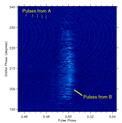
Figure 3. Radio signal from the double pulsar showing pulses from both A and B.

Figure 3 shows the radio signal strength (in a colour table where blue is weak and white is strong) from the two pulsars (they are so close together their signals are picked up in the same beam of the radio telescope). The horizontal axis is time folded at the period of pulsar B whilst the vertical axis is time labelled in the orbital phase of the binary system. Hence we can look at a horizontal line through the middle of this diagram and see that the signal from B is initially zero and then a pulse appears in the middle before it falls away to zero again. Looked at vertically we see that there are strong repeated pulses from B over orbital phases from about 195 to 230 degrees (a period of time of about 10 minutes). In fact pulses are only visible from B in this part of the orbit and another section centred on phase 28 degrees. In the background the much shorter period pulses of A can be seen. The pulse period of A appears to vary relative to that of B (resulting in the curvature of the lines in the background) because of doppler shifting due to the binary motion. Over the year since discovery the parameters of the system have been measured through timing so that, for example, the masses are increasingly accurately determined - see Figure 4.

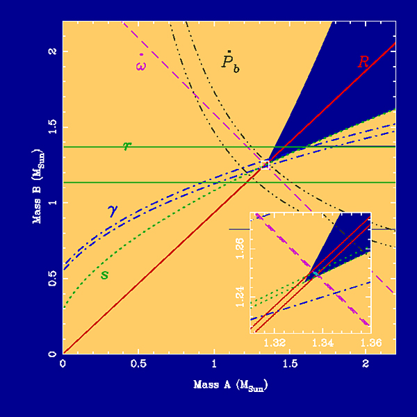
Figure 4. (a) Mass of pulsar A versus mass of pulsar B. The various observables constrain the masses to lie within the small light blue box which is shown magnified in the inset. This figure shows how well the masses were determined in December 2003. The observables indicated here are the mass ratio R, the advance of periastron (omega-dot), the gravitational redshift and time dilation parameter gamma, the Shapiro parameters r and s. Note in the magnified region each of these parameters is measured to some accuracy which is indicated by a pair of lines - the true value must lie in the intersection of these regions.

(b) As above but for December 2004. Various parameters have been determined to higher accuracy and a new parameter, the orbital decay (i.e. increase in orbital period P_b) due to gravitational wave radiation, has been added.

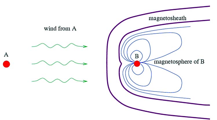
There is also a very remarkable interaction between the radio emissions of the two pulsars, which provides the most striking example of magnetospheric physics apart from the terrestrial magnetosphere itself. A powerful wind from one pulsar distorts the magnetosphere surrounding the other, forming a comet-like shape closely resembling the terrestrial magnetosheath and with many of its characteristics (see Figure 5). The diameter of the orbit, determined through radio timing, is 2.9 light-seconds, and the orbital plane lies very nearly in the line of sight; the timing-derived dynamics give an inclination within 2 degrees of 90 degrees. The line of sight to each pulsar therefore passes within 3000 km of its partner. Although the radius of a neutron star is only 10 or 11 km, every pulsar is surrounded by a co-rotating ionised and very energetic magnetosphere, which for an isolated pulsar extends to the velocity-of-light cylinder radius at which co-rotation would require a velocity of c. The magnetosphere of the millisecond pulsar, A, extends to a radius of 1084 km, while that of the long-period pulsar, B, should extend to 132,000 km, well beyond the line of sight to A at superior conjunction. A should therefore be eclipsed by B for several minutes, and an eclipse is indeed seen in every orbit. But the eclipse lasts only 30 seconds, corresponding to an 18,000 km movement of the line of sight to A across pulsar B. This was the first observation of the magnetosphere of any pulsar, but with a radius of only 9,000 km it was much smaller than expected.

We therefore see a strong influence of pulsar A on pulsar B, distorting its magnetosphere and preventing us from seeing its pulses over much of its orbit, while B's distorted magnetosphere obstructs the line of sight to A at superior conjunction. A's magnetosphere is smaller and does not cross the line of sight; it appears to be unaffected by the proximity of B. This is not surprising; the rapidly rotating A is in fact the more powerful of the two, since its energy loss by spin down is 3000 times greater (the spin down rate of both pulsars is easily measured). The detailed mechanism of energy loss from pulsars has been under discussion for many years. Originally it was thought to be simple magnetic dipole radiation at the rotation period, together with an approximately equal energy density in particles flowing out from the magnetic poles. Observations of energetic nebulae near some pulsars, notably the Crab pulsar, can however only be explained as the result of a pulsar wind streaming out along the rotation axis. The outflow apparently changes character at some distance from the pulsar, but up to now the composition close to the pulsar has been unobservable. The double pulsar binary offers the first opportunity of observing the outflow close to a pulsar.

The geometry shown in Figure 5 might apply equally well (with some changes in parameters) to the terrestrial magnetosphere and magnetopause. Around the orbit, this cometary tail points away from A, so that our line of sight to B passes through the compressed head when it is furthest away from us, and through the tail when it is closest. The orbital phases of B at which it is observable are between these two positions, when it is seen from either side of the tail. At the eclipse, pulses from A are blocked by the nose and the front half of the 'comet'. The front half of the magnetosheath is therefore opaque to radio waves, probably through synchrotron absorption. The shape of the magnetosheath seems to be well represented as a comet, although rotation of B within the magnetosheath distorts the surface, creating cusps similar to those found in the terrestrial magnetosheath, and giving the complex variations of absorption seen during the eclipse of A.

Figure 3. Cartoon (not to scale) showing the interaction between the relativistic wind from pulsar A and the magnetosphere of pulsar B. The collision of A's wind and B's magnetosphere creates a magnetosheath of hot, magnetized plasma surrounding the magnetosphere of B. The rotation of B inside this sheath modulates A's eclipse.

5.2 Cosmology

Figure 6. Illustration of how the gravitational wave background left over from the Big Bang will systematically affect the timing residuals for a sample of millisecond pulsars distributed around the sky.

Binary systems are not the only source of gravitational radiation. The events of the Big Bang should also have left over a stochastic gravitational wave background which travels through space. These waves will influence the measured pulse arrival times of pulsars on a large scale, i.e. we should detect systematic variations in the residuals for different pulsars across the sky. Hence, as shown in Figure 6, pulsars can act as the extended arms of huge gravitational wave detectors.

The effect to be measured is rather small, and it needs the precise timing of an array of millisecond pulsars to detect the expected systematic variations. Such precision has only just become available with the more wide-spread use of coherent de-dispersion. While it therefore may take another few years until this cosmological effect will be discovered, pulsars remain as the only tool to allow this discovery before the space interferometer LISA is launched and operational in about 10-15 years or so.

Figure 7. Comparison of the positions of planets orbiting pulsar PSR B1257+12 with those of the inner solar system.

5.3 Extrasolar planets

The past few years have produced a steadily increasing number of extrasolar planets discovered by optical spectroscopy. However, it should be pointed out that the first planets outside the solar system were discovered by pulsar timing around the millisecond pulsar PSR B1257+12. In 1992 Wolszczan & Frail discovered a three body planetary system which had a surprising similarity to the solar system in terms of planet distances to the central star, Figure 7. Meanwhile. there are indications of a fourth planet-size object to be found in the timing residuals. All the planets discovered with optical spectroscopy thus far have been around the mass of the solar systems gas giants but of course many people are interested in discovering Earth-sized planets. Up to now, the planets of PSR B1257+12 remain as those planets with the smallest known mass outside the solar system.

5.4 Stellar evolution - asymmetric supernova explosions

Supernova explosions are not spherically symmetric, but evidence is mounting, including the possibility of jetted gamma-ray bursts and hypernovae, that they are in fact asymmetric. Apart from evidence obtained from optical observations of very young supernovae, the strongest evidence comes from the observed pulsar velocities.

Pulsars are high-velocity objects moving at 1000 km/s or more! The average velocity of all pulsars is in fact about 450 km/s whereas the velocity of a typical star may only be a few tens of km/s How do they achieve these velocities? It seems that the answer can only be found in asymmetric supernova explosions when, during the birth of the pulsar, momentum is imparted onto the neutron star. Indeed, the explosion is so violent that if only a tiny fraction of the energy could be used to accelerate the newly born pulsar, it would be vastly sufficient to explain the observed velocities. However, the right mechanism to make use of this energy, to give the pulsar the required "kick", has not been found yet.

Figure 8. ROSAT X-ray image of the supernova remnant Puppis A. The inset shows X-ray emission detected from the central neutron star located away from the centre of symmetry of the remnant.

Up to now, only processes have been identified which could explain kick velocities up to about 500 km/s. Hence, it is important to gather more information to constrain the kick mechanism as much as possible.

The effect of kicks imparted on the neutron stars can be observed directly when a neutron star is off the centre of a supernova remnant, where we would expect it if the explosion would have been symmetric, see Figure 8.

Binary systems can also provide clues about kick mechanisms. In a double neutron star system, for instance, the second supernova explosion of the pulsar companion will change the orbital plane of the system. Geodetic precession, another effect predicted by general relativity, will occur, which can be used to fully determine the system geometry. This information can then be used to infer the direction and magnitude of the kick imparted on the companion neutron star during the explosion.

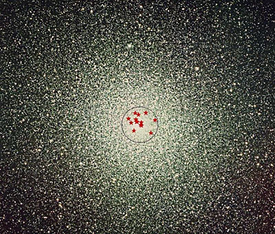
Figure 9. Anglo-Australian Telescope image of the globular cluster 47 Tuc with the position of 15 millisecond pulsars overlayed.

5.5 Probing the core of globular clusters

About 140 globular clusters are associated with our galaxy, the Milky Way. As they contain up to a million stars packed into a relatively small space, the combined starlight near its centre would make night as bright as day! The stars in globular clusters are Population II stars and hence quite old. The most massive stars must have passed their lifetime already and may have been reborn as pulsars. In fact, globular cluster are so old that one would not expect normal pulsars in the core, but only the old millisecond pulsars. Therefore, astronomers are searching such globular clusters for millisecond pulsars, and they are indeed very successful. The most impressive example is that of 47 Tucanae, Figure 9, where the research team lead by Jodrell Bank astronomers using the Parkes telescope discovered more than 20 of these exotic objects. These millisecond pulsars are used to learn more about the cluster and its evolution. 47 Tucanae is one of the most spectacular globular clusters and can be easily seen with the unaided eye in the Southern Hemisphere. At a distance of 16,000 light years it is roughly the same size in the sky as the full moon.

For 5 millisecond pulsars in 47 Tuc proper motions could be measured, Figure 10. These are in agreement with a measurement for the cluster as a whole by the Hipparcos satellite. In a few years, however, the proper motion accuracy obtained by pulsar timing will surpass that of optical measurements, and the individual motion of the pulsars in the cluster will be measured.


Figure 10. The proper motion vectors of several of the millisecond pulsars in 47 Tuc.	Figure 11. Acceleration vectors of pulsars within 47 Tuc shown in blue. The component along the observer's line of sight is shown in red.

The effects of the pulsar acceleration in the cluster's gravitational potential can however be already seen. As the pulsars are pulled towards the centre, the sign of the acceleration component along of our line-of-sight depends on the position of the pulsar relative to the cluster centre, see Figure 11. For pulsars on the near side of the centre, the acceleration is away from us; for pulsars on the far side, the acceleration is towards us. We can measure these acceleration components as a change in the apparent period slow down due to the Doppler shift caused by the gravitational pull of the cluster. In fact, since the intrinsic Pdots of millisecond pulsars are very small, the observed Pdots are dominated by these acceleration effects. The result is that the Pdots of millisecond pulsars behind the centre even become negative, while pulsars with a positive Pdot are most likely on the near side. Modelling the cluster gravitational potential we can hence infer the full 3-D positions of the pulsars in the cluster.

Figure 12. Variation of dispersion measure DM with distance R of the pulsar from the cluster centre showing that those on the far side (positive R) have higher DM implying the presence of ionised gas within the cluster.

The ability to locate the pulsars within the cluster lead to another discovery. Jodrell Bank astronomers realized that the dispersion measure is larger for pulsars on the far side of the cluster. That can only be explained if there is some substantial amount of ionised gas in the cluster. For over 40 years, astronomers have looked for gas in globular clusters at all different frequencies across the electromagnetic spectrum but no-one had been successful. It had been a mystery where the cluster gas, which was expected to be present in significant amounts, had gone. Several explanations had been put forward to explain the missing gas and amongst these were the winds from pulsars. It is somewhat ironic that the very same objects that may be responsible for the removal of most of the gas, have finally led to its detection. The clue to this discovery, i.e. the increase of dispersion measure with distance from the cluster centre is shown in Figure 12.

An animation of the pulsars in 47 Tuc putting this discovery in context.

5.6 Galactic structure

Figure 13. Illustration of the dispersion measure of a pulsar along a column of length L with electron density n_e.

Most of the applications of pulsars as tools presented up to now make use of the nature of pulsars as cosmic clocks and the timing of their signals. There are however also unique applications thanks to their emission properties which were summarised in Section 2. One such application is the study of the structure of the Milky Way.

The free electron component of the galactic interstellar medium is interacting with pulsar signals as it disperses the radio waves. The amount of dispersion is characterised by the dispersion measure DM, which is the integrated column density of the free electrons, n_e, along the line of sight of length L, see Figure 13:

We have discussed the effect of the dispersion already in the observations section where it is an unwanted complication during the observation. However, if the electron density were constant, the dispersion measure would increase linearly with the distance, providing an accurate distance estimate. In reality, the galactic electron density distribution shows some structure, for example as a result of the spiral arm structure. A more sophisticated model is therefore needed to derive the distance from the dispersion measure. In turn, if the distance is sufficiently well known, pulsars can probe the electron density by measuring the dispersion measure. Usually, an iterative process allows us to derive a distance model which is based on dispersion measures and independent distance estimates. The latest model of Galactic free electrons gives an adequate picture of the Galactic structure and also provides a distance estimate for pulsars.

This animation allows you to fly through the Galaxy with pulsars at positions as derived by the dispersion measure model.

Figure 14. The magnetic field structure of M51 shown by the white lines overlaid on an optical image of the galaxy is correlated with the spiral arm structure.

The Milky Way also exhibits a large scale, galactic magnetic field. Since we are sitting right in the plane, it is a difficult task to infer the structure of this field, which is important to understand galactic properties like star formation etc. We believe that it should be similar to field structures as seen in external galaxies like in the beautiful image of M51 by Neininger et al. shown in Figure 14.

Since we do not have this great view onto our own galaxy from outside, we have to infer the field structure from indirect measurements of its interaction with polarised radio emission. Since pulsars are unique in their property to be up to 100% polarised over almost the entire radio spectrum, they are again prime tools for these studies.

During the propagation of polarised emission through a magnetic plasma, the plane of polarisation rotates by an angle which depends on the square of the wavelength,

as illustrated by Figure 15, i.e. the effect is largest at long wavelengths and short frequencies.

Figure 15. Faraday rotation of the plane of polarisation of an electromagnetic wave as it propagates through an magnetised ionised medium.

This effect is called Faraday rotation and the rotation increases with increasing magnetic field component along the line of sight and increasing electron density. The combination of these parameter is called "Rotation Measure", RM.

where is the pitch angle of the magnetic field component towards the line of sight.

As we have seen above, the amount of rotation decreases towards higher frequencies, so that measurements at different frequencies can be used to determine the rotation measure. The combination of rotation measure and dispersion measure provides an estimate for the magnetic field component along the line of sight

The interpretation of such data is sometimes difficult, since reversals in the field direction can cancel each other, so that one measures only the average field component. Figure 16 shows such a result obtained by Han & Manchester where different field directions towards pulsars projected on the Galactic plane are shown by crosses and circles. Some sense reversal of the magnetic field towards the inner Galaxy seems to occur, but more pulsars at different distances along the same line-of-sight are needed to trace these sense reversals in more detail.

Figure 16. Looking down on our galaxy with the Sun at the intersection of the two dash-dotted lines at coordinates (0,0). The axes are labelled with distance from the Sun in kpc and, internally, by galactic longitude in degrees. Spiral arms are indicated by the dotted lines and measurements of the magnetic field directions towards various pulsars are shown as circles and crosses.

5.7 Interior of neutron stars

The matter densities found in the interior of neutron stars are so extreme that they will never be reproduced on Earth. Pulsars are hence the only way to study solid state physics under such extreme conditions. This is possible since we have seen in Part 1 that neutron stars consist of a crust and a liquid interior. The shape of the pulsar deviates slightly from a spherical shape, if the neutron star is young and spinning fast, under the influence of significant centrifugal forces. When the pulsar is slowing down in its rotation, the centrifugal forces decrease and the neutron star attempts to become more spherical. However, the rigid solid crust cannot be rearranged easily; tensions in the neutron star surface are building up. Eventually, like on Earth when tensions in the surface are released by earthquakes, it comes to a sudden, violent change in shape in the form of a "starquake" as illustrated in Figure 17.

Figure 17. The neutron star adjusts to a more spherical shape during a starquake.

During the starquake, the pulsar obtains its desired more spherical shape. The result is a concentration of the mass on a smaller radius, i.e. the moment of inertia is decreasing. As with our ice-skater from Part 1, this means a spin up of the pulsar as the angular momentum is conserved. This sudden increase in rotation rate is visible by pulsar timing, since the pulse period is suddenly decreasing. We call these rotational instabilities "glitches".

The starquake model is successful in explaining a large number of glitches in young pulsars. The relative increase in rotation rate, can be directly related to the change in moment of inertia, , and the underlying relative change in radius, via:

One problem with the model is that it needs some time until enough tension has been built up in the crust before a new starquake is released. Some pulsars, however, "glitch" much more frequently or violently than it seems possible within this model.

Figure 18. The slow down of the spin frequency of the Vela pulsar is essentially a straight line but when the overall linear decline is subtracted as in the lower panel a number of sharp steps become clearly visible.

The pulsar with the largest glitch activity is the Vela pulsar. Vela was born in a supernova explosion about 15,000 years ago and is located in the spectacular Vela supernova remnant in the Southern sky. Vela slows down rapidly and shows a large number of glitches. Figure 18 shows the spin frequency of Vela as a function of time. It is clearly visible that Vela's period of 89 ms is slowly increasing (i.e. the spin frequency decreases) as it slows down. However, superimposed on this apparent straight line, some steps are barely visible. They become much more prominent, when we subtract the overall spin down as shown in the lower part of Fig. 18.

One can notice the sudden increase in rotation frequency and a slow decay, trying to return to the overall spin down rate. The shape of this "recovery" from the glitch depends on the interior of the neutron star, so that its observation allows us to study the interior of this super-dense object. Such observations have lead to the conclusion that the interior of the neutron is indeed super-fluid as shown in the cut through a neutron star in Part 1. A recent discovery challenging this widely accepted model is briefly discussed in the next section.

Figure 19. The narrow and wide profile modes of pulsar B1828-11.

5.8 Free precession

In the early 1990's, astronomers at Jodrell Bank discovered a pulsar called PSR B1828-11 which has been monitored ever since. Recently, it became clear that the pulsar shows periodic variations in its pulse profile. It varies between a narrow and wide profile as shown in Figure 19.

Even more interestingly, this variation of the pulse profile is correlated with periodic variations seen in the rotational parameters of the pulsar, P and Pdot. This leads to the conclusion that the pulsar is freely precessing. This can happen when the pulsar is not a perfect sphere. The result is a "tumbling" of the pulsar rotation axis in space, so that we see a progressively changing cut through the emission beam which causes the changes in pulse profile.

An animation of free precession showing the slow movement of the pulsar rotation axis indicated by the green arrow.

While free precession convincingly explains the observed data of PSR B1828-11, it challenges our understanding about the interior of neutron stars. From observation of glitches we infer that the interior must be super-fluid. If this were the case, however, the precession should be damped out rather quickly, in a matter of a few days. In other words, a "tumbling liquid" is hard to maintain for a long period. However, for PSR B1828-11 we see precessional periods of 250, 500 and 1000 days, much too long to be consistent with standard theories. Ever since the discovery of free precession in PSR B1828-11, theoreticians have been reviewing the coupling of the inner liquid to the outer crust in more detail.