4. Observations of Pulsars
4.1 Instrumentation
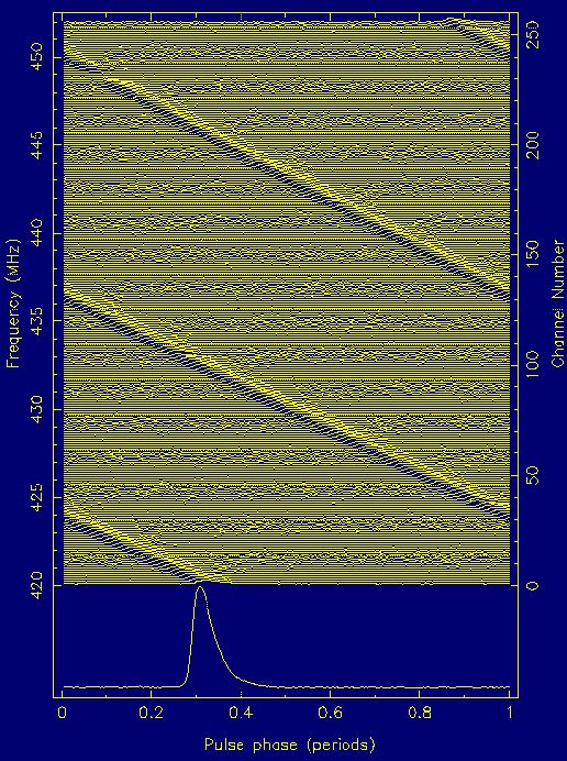
Due to their small size, pulsars are relatively weak radio sources. Therefore, the largest radio telescopes in the world are usually needed to observe them. As we have seen, pulsars emit their largest intensity at low radio frequencies around 400 MHz. In particular at such frequencies, however, the pulses suffer from propagation effects when they travel to Earth through the interstellar medium.The most obvious effect is that of "dispersion". By interacting with the free electrons in the interstellar medium, pulses at lower frequencies are delayed. In other words, pulses emitted at higher frequencies arrive earlier than those emitted at lower frequencies. This effect is shown in Figure 1 which shows pulses at different, adjacent radio frequencies.
 |
|
Figure 1. Real data showing the dispersion effect in the progressive delay of pulses to higher frequencies. |
The bottom of Figure 1 shows the pulse profile obtained after delaying the high frequency pulses until the lowest frequency arrived before summing up all frequency channels. We call this process to correct for dispersion "de-dispersion". If the delay would not have been accounted for, the summed pulse would have been blurred and smeared. If the delay is too big, the pulses may become undetectable. The dispersion delay measured in milliseconds increases at lower frequencies as
![]()
where the ![]() low and
low and ![]() high
are the lower and higher frequencies, respectively, measured in MHz.
The constant
DM is called the "dispersion measure" and increases with distance and electron
density between Earth and pulsar (see parts 4.4 and 4.5 below) and is measured in units of parsecs per cubic centimetre (a distance and an electron
density as you shall see later).
high
are the lower and higher frequencies, respectively, measured in MHz.
The constant
DM is called the "dispersion measure" and increases with distance and electron
density between Earth and pulsar (see parts 4.4 and 4.5 below) and is measured in units of parsecs per cubic centimetre (a distance and an electron
density as you shall see later).
Observations are always made with a finite bandwidth, BW. The larger
the bandwidth, the more emission can be received, making the observations
more sensitive. Hence, one usually attempts to maximise the bandwidth.
At the same time, however, the dispersion smearing increases and the pulses
observed at a frequency ![]() in MHz would be blurred by
in MHz would be blurred by
![]() seconds per
MHZ of bandwidth
seconds per
MHZ of bandwidth
if no de-dispersion were done. The easiest way is usually to follow the example of the above plot and to split the total bandwidth, BW, into a number of smaller channels. The signals are then detected and delayed before summing as described above. Of course, there is still dispersion smearing in each of the smaller channels, so that the channel width is chosen depending on observing frequency and aim of the observations. We will review another de-dispersion method, which removes dispersion completely, below.
The sensitivity of the observation, or the "signal-to-noise" ratio describing the strength of a signal compared to random noise, depends on more parameters than just the bandwidth of the receiving system:
- The size of the telescope matters, which is described by the "gain" parameter. The larger the telescope, the larger the gain, G.
- Each piece of equipment involved produces a random thermal noise signal. This is the reason why one tries to cool receivers to temperatures of only a few degrees above absolute zero. Any remaining thermal noise signal is described by the system noise temperature, Tsys.
- Thermal noise is a random signal, while the pulsar signal arrives periodically with the pulsar period. Averaging ("integrating") the received signals over a period of time, will therefore reduce the random noise relative to the real signal. Hence, the signal-to-noise ratio, "SNR" or "S/N", increases with integration time, tint.
- A simple receiver system is only sensitive to one of two orthogonal polarisation directions. One usually combines two such systems, to measure the intensity in both directions. Effectively, one then increases the used bandwidth by a factor equal to the number of received polarisations, Npol (max. 2).
|
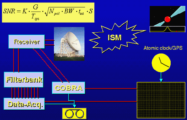
Figure 2. Schematic of pulsar observing system. The pulses emitted by the pulsar (upper right) propagate through the interstellar medium (ISM), before being picked up by a telescope and the installed receiving system. In a standard approach the total bandwidth is split into smaller channels by a filterbank (for each polarisation). The signals of each filterbank are acquired by a data acquisition system and recoded along with information from the observatory's atomic clock which is synchronised to an international time standard with GPS. |
 |
 |
|
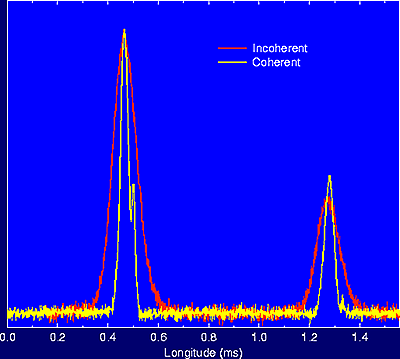
Figure 3. Illustration of the advantages of coherent dedispersion in observations of PSR B1937+121. |
Figure 2 also shows another instrument, COBRA, which is being commissioned
at the Jodrell Bank Observatory to replace the previous filterbank system.
This new system uses a de-dispersion method called "coherent de-dispersion"
which is able to restore the original pulse shape completely. Although
this method requires substantial computing power, it removes all dispersion
smearing, producing much sharper pulses. Sharper pulses allow us to measure
the arrival times of pulses to a much higher precision which is important
for pulsar timing (see next section). The superiority of coherent de-dispersion
over the "incoherent" filterbank method is shown for the pulse profile
of PSR B1937+21 in Figure 3.
4.2 Pulsar timing
 |
|
Figure 4(a). The residuals between a good model and actual pulse arrival times scatter around zero. |
 |
|
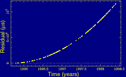
Figure 4(b). Increasing residuals due to wrong spin-down rate. |
 |
|
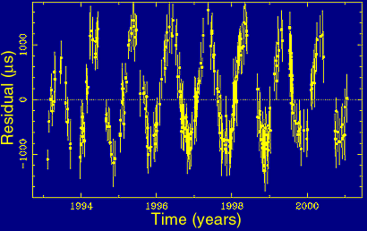
Figure 4(c). Deviation with one year period due to inaccurate position. |
 |
|
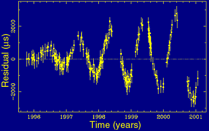
Figure 4(d). Deviation with one year period and increasing amplitude due to inaccurate proper motion. |
We have already discussed the effects of dispersion on the arrival time of pulses. Much more fundamental is however, that the arrival time must be different for any telescope and must also change with time of day and time of year as any given telescope is moving in space due to the Earth's rotation and movement around the Sun. For our experiments we should refer to the arrival time at a point in the solar system which is at rest. Such a point is the system's centre of mass, the so-called solar system barycentre.
If the pulsar is not too distant, we can measure a parallax effect in the time of arrival providing a direct measurement of the pulsar distance. (To be precise, we measure the curvature of the incoming electromagnetic waves!)
General relativity predicts additional delays when the pulse is propagating through gravitational potentials like that of the Sun.
All these effects have to be taken into account before we can attribute changes in arrival time due to physical effects by the pulsar. We can summarise them in the following equation which describes the transformation of the measured arrival to the time of emission in the pulsar frame.
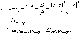
The first term refers to a certain chosen epoch t0 as reference, the second term describes the transformation to the solar system barycentre (r and s being vectors pointing from the telescope to the pulsar and Sun, respectively), the third term accounts for dispersion with D being a constant depending on the dispersion measure, while the fourth terns becomes relevant when the pulsar is close (d is the distance of the pulsars), so that parallax effects are important. The fifth term describes the aforementioned effects predicted by general relativity.
Things become more complicated if the pulsar has a binary companion. In that case, most of the effects present in the solar system will have to be accounted for in the binary system as well, which is indicated by the last two terms. Binary pulsars are discussed in more detail in the next section.
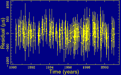
Accounting for all possible effects including the pulsar spin down, we should be able to predict the arrival times and to compare these predictions with actual measurements. These differences between model predictions and observations called "residuals" are plotted versus time and should vary randomly around zero, as shown in Figure 4(a), if the model is correct.
Deviations from a random appearance indicate unmodeled effects. An inaccurate assumption about the pulsar spin down, for instance, leads to an increasing deviation from the expected arrival time as in Figure 4(b).
If the assumed pulsar position is inaccurate, our transformation to the solar system barycentre will be wrong too, creating a deviation from the expected arrival time that depends on the position of the Earth in its orbit. Hence, the deviation will have a sinusoid shape with the period of one year, Figure 4(c). The amplitude then depends on the amount by which the assumed position is wrong.
If the pulsar exhibits some proper motion that is not accounted for, its position must become increasingly inaccurate, producing an one-year sinusoid with increasing amplitude, Figure 4(d).
In an iterative procedure during which such deviations are identified, the pulsar model is improved until the residuals show the expected random distribution of Fig 4(a). Using this method, we can determine the pulse period and the pulsar spin down as well as astrometric parameters like position and proper motion to an incredible accuracy. The accuracy achievable scales with the pulsar period, so that the best results are obtained for the shortest periods i.e. the millisecond pulsars. The pulse period of PSR B1937+21 is, for instance, measured to be:
Similarly, positions and proper motions are measured to accuracies of
microarcseconds and microarcseconds per year, respectively. This is better
than any other method currently available in astronomy.
4.3 Timing binary pulsars
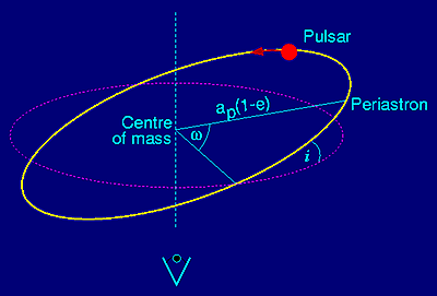
The presence of a companion to a pulsar affects the arrival time of the pulses at Earth. This is (apart from additional relativistic corrections to be discussed later) due to the binary motion of the pulsar illustrated in Figure 5 and described by the 5 Keplerian parameters: orbital period; projected semi-major axis of the orbit; eccentricity; and longitude and epoch of periastron.
These Keplerian parameters can be derived with pulsar timing in a similar
way as is done for spectroscopic binaries in the optical regime. Figure
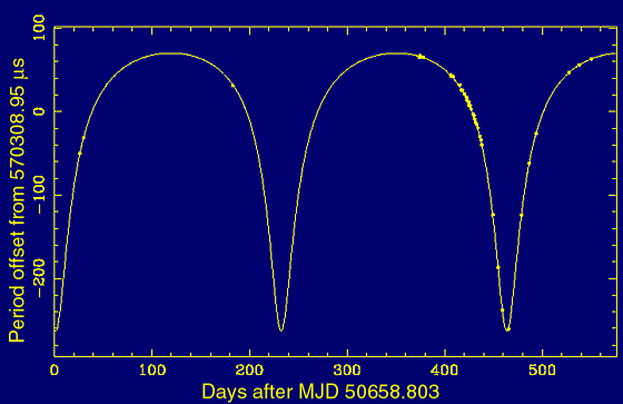
6 shows, for instance, the variation of the 570-ms pulse period as measured
for the recently discovered PSR J1740-3052, which has the heaviest companion
of any known pulsar in a 230-day orbit.
 |
 |
|
Figure 5. Binary parameters. Observer views from below. |
Figure 6. Variation of pulse period for pulsar PSR J1740-3052 due to binary motion. The dots are observed data and the line is the best-fit model. |
The companion mass can be estimated from the mass function which is
derived from Kepler's 3rd law and combines the observed Keplerian parameters
with the pulsar and companion mass. Using G as the gravitational constant,
ap as the projected semi-major
axis of the orbit, Pb as the orbital period and mp
and mc as the mass of the pulsar and its companion, the mass
function f is computed as:
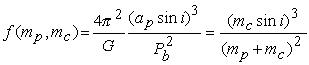
The left hand side consists of observable parameters, which can be related to the masses on the right hand side.The inclination angle of the orbit, i, is in principle unknown, but by assuming an inclination of 90 deg, one can at least derive a lower limit on the companion mass. In the case of PSR J1740-3052, this is an amazing 11 solar masses. The nature of the companion is still unclear, and it has been speculated as to whether this system could be the first pulsar-black hole binary system discovered.
The Keplerian parameters would describe the binary motion completely, if Newtonian physics were the correct theory of gravity. Albert Einstein has demonstrated that this is not the case, when he introduced general relativity. If general relativity, or any other theory of gravity deviating from Newtonian physics for that matter, is correct, we need additional parameters to describe the relativistic corrections needed to be made to the Keplerian motion. These "post-Keplerian" parameters can also be determined by pulsar timing and can then be compared to predictions by general relativity or any other theory. The next section discusses how pulsars are the best tools to perform these relativistic tests.