1. Properties of Pulsars
1.1 The discovery of pulsars
Shortly after the discovery of the neutron by Chadwick in 1932, two astronomers, Baade & Zwicky, proposed that during Supernova explosions small, extremely dense objects could be created in the centre of the exploding star. They suggested that the enormous pressure occurring in the centre of the explosion would be sufficient to enable an "inverse beta-decay" during which electrons and protons are combined to neutrons and neutrinos. Neutrinos could leave the star to carry away a substantial amount of energy, leaving behind a very dense object consisting mostly of neutrons. They called these objects accordingly "neutron stars".Five years later, Oppenheimer (who later lead the Manhattan project) & Volkov were the first to calculate the expected size and mass of these newly predicted objects. Based on quantum mechanical arguments they computed that neutron stars should have a diameter of about 20 km while containing 1.4 times the mass of the sun. Given this extremely small size expected for these objects, astronomers therefore considered it to be impossible to ever detect neutron stars and hence to verify the predictions by Baade & Zwicky.
 |
|
Figure 1. Copy of the chart recorder output on which are the first recorded signals from a pulsar. |
The situation changed dramatically in 1967. Meanwhile a new window had been opened up for astronomers, the radio window. It was in summer 1967 when a research student, Jocelyn Bell, was working on her PhD thesis at Cambridge under the supervision of Anthony Hewish. They wanted to study the intensity variation of quasars, which were discovered only a few years earlier. After constructing a radio telescope dedicated to monitor the sky for intensity variations, Jocelyn Bell came across a signal which originated from a certain location in the sky, RA B19:19:36 - DEC +21:47:16. The signal was highly periodic with a periodicity of 1.337 seconds. Figure 1 shows the discovery recording.
The astronomers were puzzled by this discovery and wanted to establish its nature before they made it public. Indeed, one possibility that was seriously considered was that of a signal sent by extra-terrestrial intelligence. Soon, however, the team discovered more such periodic signals, and it seemed highly unlikely that one would suddenly receive signals from many different civilisations at once. Moreover, a period variation due to a Doppler effect caused by the moving planet of a possibly transmitting civilisation was not discovered. A natural origin of the signal was hence concluded.
1.2 The nature of pulsars
A journalist finally invented the name "Pulsar" for these objects, standing for "Pulsating Radio Source". Three possible explanation were put forward in the publication reporting the discovery. A pulsar could be- an oscillating object (similar to intensity variations of Cepheids in the optical),
- an orbiting object (i.e. a companion eclipsing a radio source) and
- a rotating object (like a rotating lighthouse).
 |
|
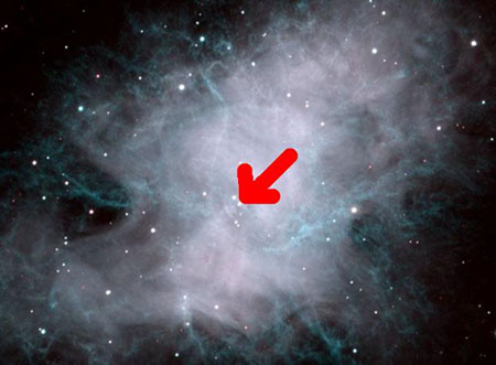
Figure 2. Optical image of the Crab nebula (NOAO). The arrow marks the position of the pulsar. |
The Crab Nebula (Figure 2; also called M1 as it was the first object in Messier's famous list) is the visible remnant of a supernova explosion witnessed by Chinese astronomers in A.D.1054. The nebula had been in the focus of discussions before, since its brightness was hard to explain given the nebula's age. It was suggested that a mysterious star visible in the centre (see arrow in Figure 2) was responsible, but the star did not fit any known category. It happened that in parallel to the discovery of pulsars, Thomas Gold (1968) had proposed that the nebula could be powered by a highly magnetised neutron star. After the discovery of pulsars, Staelin & Reifenstein (1968) observed the nebula for pulsed radio emission. They discovered high intensity pulses originating from the central "strange" star, identifying it as a pulsar. It turned out later, that these "giant pulses" which they observed, occur every two minutes or so, and that the true pulse period was in fact as short as 33 milliseconds.
The short period of 33 milliseconds ruled out white dwarfs for being
pulsars: radial oscillations were estimated to be only possible for periods
larger than 1 second. Similarly, a maximum radius of a rotating object
can be estimated from requiring equality between centrifugal forces and
the gravitational force at the equator. If R is the radius of the pulsar,
M its mass, and ![]() the
the
angular velocity and P the pulse period, we obtain for a test
mass m at the equator:
Periods for radial oscillations of neutron stars were predicted to be larger than 1 second and were hence incompatible with the periods of the first discovered pulsars. Finally, another property of pulsars, also most easily observed in the Crab pulsar, provided the final clue. It was noticed that the period of pulsars slowly increases, for the Crab pulsar by as much as 36 nanoseconds per day. This property is not expected for the model of an eclipsing binary, where due to the loss of energy one would in fact expect the companions to come closer, reducing the pulse period. However, a slow-down of the period is indeed expected for a rotating object. The problem was finally solved: pulsars are rotating cosmic light houses.
Pulsars are named according to their celestial coordinates. Using the equatorial system, the name is composed from hours and minutes of right ascension and degrees (and minutes) of declination, preceeded by a leading "PSR" for "pulsar". As the Earth axis is precessing, the equatorial coordinate system changes slowly and we have to indicate the epoch we refer to. For all newly discovered pulsars today, J2000 coordinates are chosen and we write, for instance, PSR J1022+1001. In the past, coordinates referred to epoch B1950, and well studied pulsars are still known under their B1950 names (not including minutes of declination), e.g. see PSR B0329+54 below.
Pulsars spin extremely fast, typically around once per second but spanning a range of four orders of magnitude. The sounds below are from the brightest pulsars in the sky, recorded using some of the largest radiotelescopes in the world.
 PSR
B0329+54: This pulsar is a typical, normal pulsar, rotating with a period
of 0.714519 seconds, i.e. close to 1.40 rotations/sec. PSR
B0329+54: This pulsar is a typical, normal pulsar, rotating with a period
of 0.714519 seconds, i.e. close to 1.40 rotations/sec. |
| PSR
B0833-45, The Vela Pulsar: This pulsar lies near the centre of the Vela
supernova remnant, which is the debris of the explosion of a massive star
about 10,000 years ago. The pulsar has a period of 89 milliseconds, rotating
about 11 times a second. |
| PSR
B0531+21, The Crab Pulsar: This is the youngest known pulsar rotating about
30 times a second. |
| PSR
J0437-4715: This is a millisecond pulsar now rotating about 174 times a
second. |
| PSR
B1937+21: This is the fastest known pulsar, rotating with a period of 0.00155780644887275
seconds, or about 642 times a second. The surface of this star is moving
at about 1/7 of the velocity of light and illustrates the enormous gravitational
forces which prevent it flying apart due to the immense centrifugal forces. |
1.3 Spin-down, magnetic field and the age of pulsars
The electromagnetic radiation emitted by pulsars is taken from the rotational energy of the neutron star. From the observations of the Crab nebula, Gold deduced that the pulsar must be highly magnetised. Therefore, most of the electromagnetic radiation takes the form of low frequency magnetic dipole radiation. We can equate the power of magnetic dipole radiation with the loss in rotational energy,![]()
where ![]() is
the change in spin energy, I the pulsar's moment of inertia of the order
of 1038 kg m2,
is
the change in spin energy, I the pulsar's moment of inertia of the order
of 1038 kg m2, ![]() and
and ![]() the
spin frequency and its change. mB is the magnetic dipole moment
of the pulsar, and
the
spin frequency and its change. mB is the magnetic dipole moment
of the pulsar, and ![]() the angle between the rotation and magnetic axis.
the angle between the rotation and magnetic axis.
We derive a simple expression for the evolution of the spin frequency.
The spin frequency decreases with a power law index, n, which we call the braking index. If the spin-down is purely due to magnetic dipole radiation the index is expected to be 3.
The spin frequency evolution of course also predicts the evolution of the spin period. Assuming a braking index of 3 and assuming that the initial spin period is much smaller than the currently observed pulse period, we can estimate the so-called "characteristic age" of the pulsar.
![]()
which uses the period P and the period derivative ![]() only.
only.
These are usually very reasonable assumptions (see later), and applying the equations to the Crab pulsar we derive an age of 1257 years. This is not too different from the true age of the pulsar, which we know must have been created during the supernova explosion in A.D.1054. For astronomical purposes this is certainly a surprisingly good precision.
As the spin-down is related to the magnetic field, its strength B can be estimated from the observations as well:
using c as the speedof light, in addition to the definitions made before. For the typical properties expected for neutron stars we derive magnetic fields of the order of 108 Tesla. As it is general practice in pulsar astronomy (or habit, to be precise!) to quote magnetic fields still in Gauss, we will do so in the following, i.e. the typical magnetic field is of the order of 1012 Gauss. This is twelve orders of magnitude (i.e. a factor one million million) larger than the Earth's magnetic field, and at least five orders of magnitude larger than any magnetic field ever created in a laboratory for fractions of a second. Interestingly, the field strengths estimated are in surprisingly good accordance what is needed to explain the brightness of the Crab nebula. Moreover, X-ray observations of neutron stars have later resulted in independent measurements of the field, confirming that these models are simple but surprisingly accurate.
Astronomers have developed the Hertzsprung-Russell diagram to describe the life cycle of stars. Radio astronomers use a similar diagram to discuss the life of a radio pulsar, the P-Pdot diagram, Figure 3. In such a diagram we plot the period derivative (the rate of change of the period in units of seconds per second - commonly called Pdot after the mathematical notation for rates of change in which a dot is placed over the relevant symbol, in this case a P) versus the pulse period on a logarithmic scale. (Similarly, one can plot the magnetic field versus period as we will do later.) Since both characteristic age and surface magnetic field are functions of period and period derivative, lines of constant age and magnetic field are straight lines in such a P-Pdot diagram.
 |
|
Figure 3. A P-Pdot diagram. |
Pulsars are born with small periods and slow down fast in their rotation when they are young (i.e. they exhibit a large Pdot). Hence, pulsars are born in the upper left part of the diagram. This is also the region where we find those pulsars which are still associated with supernova remnants. These remnants fade and are not detectable anymore after a few hundred thousand years or so. Therefore, older pulsars with typically ages of a few million years can be found in the centre of the diagram. If pulsars slow down further, conditions to create radio emission apparently cease, and the longest period known for any pulsar is just about 8 seconds. Eventually, pulsars that have a companion may have the chance for a second life, appearing as "recycled pulsars" in the lower left part of the diagram (see Section 2 of these notes).
1.4 Size, Mass and Structure of Pulsars
Oppenheimer & Volkov used quantum mechanics to predict a mass of 1.4 solar masses for a neutron star. The exact value depends on the Equation-of-State (EOS) which describes the internal pressure and density of an object depending on the mass, defining its radius, see Figure 4.
 |
|
Figure 4. The mass-radius relation for pulsars. |
The EOS is not very well known for such high densities as encountered in neutron stars. From observations of binary pulsars (see later) we can however measure the mass for a number of neutron stars. The observations show an average mass of 1.35 solar mass, which is again very close to theoretical predictions, Figure 5.
 |
|
Figure 5. Measurements of neutron star masses shown as dots with uncertainties as horizontal error bars. |
 |
|
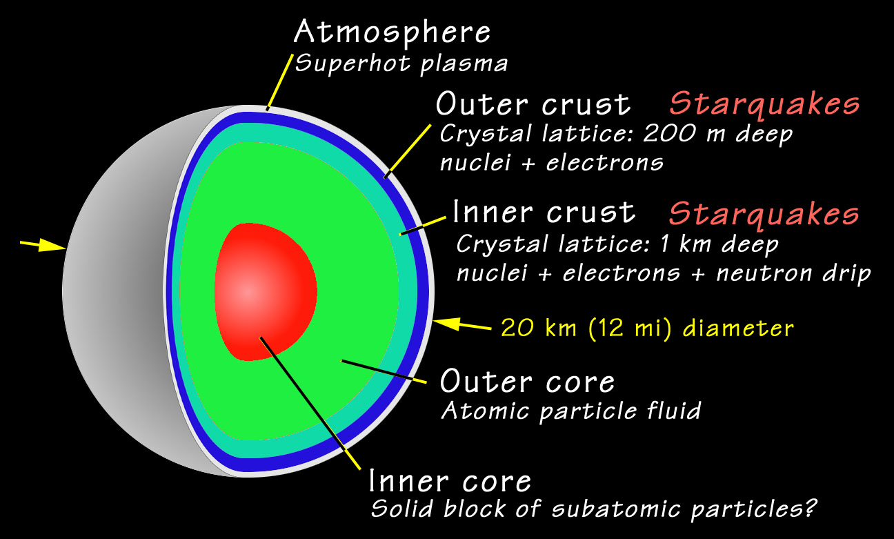
Figure 6. Cross section through a neutron star. |
The fact that observations agree impressively well with the theoretical
predictions give good confidence that we indeed understand the basic structure
of these super-dense objects. As shown in Figure 6, a neutron star has
an outer crust consisting of a crystal lattice of iron nuclei and electrons.
Going deeper inside we pass an inner crust and come to a point ("neutron
drip") where most electrons and protons form neutrons. The core is hence
made of an ensemble of neutrons acting like a fluid with the unusual properties
of being super-fluid and super-conducting (no frictional or electrical
resistance). The pressure in the core is as high as 1014
grams per cubic centimetre. Depending on the EOS there may be an inner
core, where nuclear particles are even dissolved into bare quarks. The
neutron star is surrounded by a hot plasma of a few million Kelvin. The
height of the atmosphere is only a few cm, but its effects can be studied
in X-ray spectra of neutron star surface emission. Such observations also
allow to infer the size of the emitting surface, which confirm the theoretical
size estimates.
 In
order to comprehend their relative sizes take a flight past the Sun and
Earth and approach a red sphere the size of a pulsar. In
order to comprehend their relative sizes take a flight past the Sun and
Earth and approach a red sphere the size of a pulsar. |
The following animations demonstrate that pulsars concentrate so much mass that they are almost black holes. In fact, if a pulsar would have only twice as much mass, a collapse to a black hole could probably not be prevented. Both animations are based on correct calculations in the frame work of general relativity, i.e. the theory of gravity introduced by Albert Einstein, describing how light is bent in the gravitational field near the pulsar surface.
| In
the first animation, you can watch the distorted sky beyond the pulsar
while you circle around it. The Earth's continents have been mapped onto
the surface to indicate the rotation. [From here] |
| In
the second animation you are moving on the surface of the neutron star
(which cannot be recommended due the strong fields and the temperature
of a few million degrees Kelvin!). Again, you can see the distorted sky.
In principle, the light can be bent around the surface so that you can
see the back of your own head! [From here] |
1.5 The Birth Of Pulsars
The discovery of young pulsars near supernova remnants is the final confirmation that Baade & Zwicky were absolutely right when they predicted neutron stars more than 30 years before they were finally discovered.
 |
|
Figure 7. Three phases during the life of a star: virtually all its life is spent in the nuclear burning phase, following the exhasution of nuclear fuel it collapses and a supernova explosion leaves behind a neutron star. |
As illustrated in Figure 7, during the life of a star the gravitational force is balanced by the radiation pressure created by nuclear fusion inside the star. As soon as all available fuel is used up, nuclear fusion ceases and no force is present to balance gravitation any longer. The star collapses. The central regions are compressed creating the neutron star. Quantum mechanics predicts that the newly formed neutrons produce a pressure caused by the Pauli exclusion principle for fermions, which prevents that neutrons are further compressed (unless the mass is so large that collapse continues to a black hole). Matter from the outer layers that is still in-falling to the centre hits the neutron star, bounces back and creates an enormous explosion when colliding with other in-falling matter. This explosion produces the light which can outshine entire galaxies. For the central part, mass had been concentrated in the neutron star on much smaller radius.
 |
Like the spin-up of an ice skater during a pirouette when pulling the arms towards the body, the conversation of angular momentum of the slowly rotating progenitor star creates the small birth periods of pulsars. Similarly, magnetic flux is conserved explaining naturally the extreme large surface magnetic fields of pulsars.
The discovery of neutron stars showed that our basic understanding of
quantum mechanics and its predictions for stellar evolutions is correct.
This was acknowledged with the Nobel Prize in Physics in 1974 for the discovery
of pulsars.
 |
|
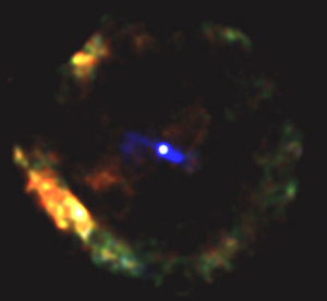
Figure 8. A supernova remnant seen in X-rays by the Chandra Observatory. |
While astronomers had been pessimistic about ever been able to observe neutron stars after Baade & Zwicky's predictions before pulsars were actually discovered, advances in technologies have also allowed direct observations today: a neutron star is slowly cooling down with a typical surface temperature of about a million Kelvin. Modern X-ray satellites like XMM-Newton or CHANDRA can nowadays detect the emission of the hot surface (Note that the maximum of the Planck curve for a body of such temperature is indeed expected at X-ray frequencies). The image in Figure 8 is such a direct observation of a neutron star in the centre of supernova remnant. The emission that forms part of a circle around the bright neutron star at the centre is from gas which has been heated to millions of degrees Kelvin in the shock wave marking the interaction between material ejected from the supernova and the external interstellar medium.
In the next section we will go on to look at how pulsars are sources
of radio emission, the primary way in which we discover them and investigate
their properties.