2. Geometry of lens systems

Deriving the geometry of a lens system - Method 1 (the Lens Equation)

Consider the idealised system shown in Figure 2.1, where the symbols D_s, D_l and D_ls are used for the distance from the observer to the background source, the observer to the lens and the lens to the source respectively.

Figure 2.1. Geometry of a gravitational lens system. Light from the background object at Q follows the trajectory shown by the blue arrow, deflecting by angle at P and then travelling to the observer. As a result, the observer sees the image at Q' rather than Q. Note that all the angles are very small, and have been exaggerated for clarity by a factor of about a million in this diagram.

All of these deflection angles are very small. Therefore we can use an important result from geometry; for an isosceles triangle (one with two sides of equal length) with two very long sides and one short side, the product of the small angle between the long sides and the length of one of the long sides is equal to the length of the short side, provided that the angle is expressed in radians. Luckily this is already the case in the equation we saw earlier for the deflection angle in a gravitational field.

You can therefore see that the length OQ is just D_s, and OQ' is D_s. [If you're worrying that these triangles are not isosceles but rather are right-angled then you can think about the isosceles triangles which would be formed by reflecting these right-angled triangles in the horizontal plane - the angles at the apex of these triangles are then 2 and 2 but the lengths at the bases are also doubled so the same formulae result. Alternatively if you are happy with trigonometry you could consider the tangent of the angles and remember that tangents of small angles are equal to the angle itself measured in radians.]

Now consider the triangle PQQ'; you can derive from this triangle that the distance QQ' is D_ls.

Obviously OQ + QQ' = OQ', and so

D_s + D_ls = D_s

so rearranging, we finally get

= (D_s/D_ls) - (D_s/D_ls)

which is known as the "lens equation".

If we were to plot against we would therefore get a straight-line graph with gradient (D_s/D_ls) and intercept - (D_s/D_ls) .

So far we have not included any information about the physics of exactly how the light gets deflected. We can do this quite easily if we remember for a point mass lens that

= 4GM/bc²

and the distance of closest approach, b, is just D_l; therefore = (4GM/c²) x 1/(D_l) - in other words, the deflection angle decreases for rays which pass a greater distance from the centre of the lens.

Obviously the point mass is not a particularly good representation of a real galaxy. Real galaxy "lenses" have a much slower falloff of deflection angle with distance, and in fact a constant (call it ₀) which just reverses sign as the light path goes one side or the other from the galaxy centre is a good approximation. This is known as the "isothermal" model, and corresponds to a surface mass density which falls off as 1/r, where r is the distance from the centre of the galaxy. The abrupt change in corresponds to a singularity in the mass distribution in the centre, and such galaxies are known as "singular isothermal ellipsoids", or "singular isothermal spheres" for those that are spherical in distribution rather than elliptical.

1. Using the equations given so far, work out an equation for the angular size for the Einstein ring produced by a point mass M in terms of the distances to lens and source. You will need the lens equation, remembering that for the Einstein ring =0, and Einstein's equation for light deflection by a point mass.

2. Try the same exercise for a galaxy, modelling it instead as a singular isothermal sphere.

For an image to be formed, we must demand that both equations - the lens equation and our idea of the dependence of and - are satisfied simultaneously. You should convince yourself that in this simple model, either one or three images of the background source can be formed, depending on how close the lines of sight are to the lensing object.

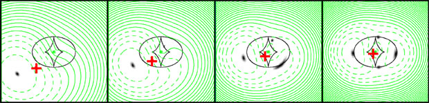
The gravitational lens simulator

In practice, more complicated analysis in two dimensions allows the possibility of five lensed images, provided that the lines of sight to background source and lens are close enough. The gravitational lens simulator available on the web from Jodrell Bank allows you to investigate the types of images that are seen for different positions of the source compared to the lens centre. Look especially for the following, see Figure 2.2:

Only one image is formed if you place the source very far from the lens.
As you bring the source closer, the image distorts and stretches. The image appears some way away from the line of sight to the source, because of the deflection angle ; investigate how this varies with distance from the galaxy for the point-source and isothermal-ellipsoid models.
As the source crosses the outer black line, a second image begins to appear close to the lensing galaxy. This image is in general much fainter. A third image also appears in the centre, as you expect from the earlier analysis, but it is so faint that it cannot be seen. (In the case of the lenses considered here, the third image is in fact demagnified to zero).
As the source crosses the inner black, diamond-shaped line, a further two bright images appear. They are initially merged together in an arc, but separate as the source moves closer to the galaxy or as the galaxy ellipticity increases. There are in fact a total of five images, but once again the central image is extremely faint and only four images are seen in practice.

Figure 2.2. This figure illustrates the images (in grey) formed as a source (the red cross) is brought steadily closer to a galaxy (blue dot). As the source crosses the outer ring, two images begin to appear (one is on the top right edge of the diamond); on crossing the inner diamond, four images are seen (two are initially smeared together).

Use the simulator to investigate the dependence of the images' appearance on the parameters in the simulation. In particular, notice the following: (i) How does the galaxy ellipticity change the types of image seen as you move the source closer to the galaxy? (ii) What effect does the Einstein radius have on the simulation?

Parity

Individual images within the gravitational lens system form, as we have seen, with different magnification. Some of the images also have different parity, a quantity which can be positive or negative. A positive-parity image of a Z-shaped source would appear as a Z-shaped image (although possibly distorted), whereas a negative-parity image would appear S-shaped. In general, negative-parity images form closer to the centre of the lens. For example, in a two-image system the fainter image closer to the centre of the lens has negative parity, and the brighter, more distant image has positive parity.

Deriving the geometry of a lens system - Method 2 (Fermat's principle)

There is a second, rather elegant way to examine the geometry of a gravitational lens system. It is by the use of Fermat's principle, originally stated by the French physicist Pierre de Fermat (1608-1665). In the form he originally stated it, it reads:

The actual path between two points taken by a beam of light is the one which is traversed in the least time.

The more modern formulation, which is needed in studies of gravitational lensing, reads:

The actual path between two points taken by a beam of light is the one which is an extremum - that is a maximum, a minimum or a saddle point.

A saddle point is strictly speaking neither a maximum or minimum, but as its name implies is a locally flat area similar to that at the centre of a saddle - it resembles a maximum in one direction (across the horse) and a minimum in another (along the horse). In all three cases the main point is that the difference in light travel time which results from going a small distance from the extremum is vanishingly small. In the language of calculus, this means that the first derivative of the path with respect to small deviations vanishes.

For light propagating through a uniform medium from point A to point B Fermat's principle is very simple. The light ray will just follow the path of minimum time - in other words, a straight line.

For light propagating through a gravitational lens, the situation is different. Suppose that the source, the lens and the observer are all in a straight line. If the light now follows a "straight line" it has to go through the centre of the lens, which contains a large gravitational field. The effect of this field is to retard the light as it struggles out, and more time is taken. The shortest path would therefore be one which avoids the centre of the lens and is deflected to reach the observer, but not so far that a large overhead is incurred by travelling a longer distance. The resulting compromise corresponds exactly to the light path which we derived earlier using the lens equation. In practice, not only the minimum-time path will be followed but, due to the complicated nature of the lens, images also form which have followed maximum paths and paths corresponding to saddle points.

Try the gravitational lens simulator again, but this time selecting the option to "Plot Fermat surfaces". These purple lines are contours of constant light travel time; in other words, light from the source which has gone through any point on each connected line will take the same time to reach the observer. Repeat the previous lens simulation exercise, but this time note that:

for the source far from the lens, the image is a Fermat minimum path as you would expect
as the source approaches the lens, other images form, all of them at Fermat extrema. What type of Fermat extremum does each new image form at?

Jim Lovell (U. Tasmania, Australia) produced this animation of a background radio source at different points behind a gravitational lens. In this case the background source is extended, and complex structure including an Einstein ring is formed for close coincidences of the lines of sight.

Types of lens system

Any concentrated mass can in principle act as a gravitational lens. Whether multiple images are visible depends on the concentration of mass at the centre of the lens, the central surface mass density (a surface density is the mass per unit area, normal densities are volume densities i.e. mass per unit volume). Only above a critical value of central surface mass density (CSMD) will the characteristic multiple imaging be seen.

Table 1 shows the three major types of lensing which are astronomically important (adapted from a similar table in a review article by Refsdal & Surdej). In most of this course we will consider only lensing by single galaxies. However, lensing by stars ("microlensing") and lensing by clusters of galaxies will be discussed in section 7.

Table 1. Types of lensing.

Lens	Lensed object	Central surface mass density	Einstein radius
Single galaxy	Usually quasars; can be background galaxies	For normal lensing galaxies, a few times critical CSMD	About 1 arcsecond
Single star (or massive object, e.g. black hole) in our galaxy	Background star in our galaxy or Magellanic Clouds	Vastly greater than critical CSMD (lensing object very compact)	About 1 milliarcsecond (very hard to resolve)
Cluster of galaxies	Many background galaxies	About critical CSMD in cluster centre, stretching and distortion also seen	Tens of arcseconds

As was derived above , the angular radius (in radians) of an Einstein Ring is given by

²=4GMD_ls / c²D_lD_s .

Use this formula to confirm the orders of magnitude of the Einstein radii presented in Table 1. You will need to choose appropriate values for the various distances and lens masses.

In the next section we will discuss the way in which we search for lenses.

Answers to questions

Answer to question

Angular size is given by ²=4GMD_ls / c²D_lD_s.

From the geometry (fig 2.1), b=D_l, so the equation for a point source becomes =4GM/D_lc². Combining this with the rearranged lens equation: =D_s/D_ls gives the result.

2. Try the same exercise for a galaxy, modelling it instead as a singular isothermal sphere.

Answer to question

=D_ls₀/D_s

This one is easier: the singular isothermal model has a constant deflection, which we call ₀. Substituting this into the lens equation (with =0) gives the required result.